R Module
Jake Rothschild, Behavioral Development Lab
Overview
This document will teach JPAL employees the basics of R. It focuses on the Tidyverse method of programming and the ggplot package for graphics. Please note that while Tidyverse is a commonly used and widely accepted method of R programming, there are other viable methods.
This module focuses on the following uses of R:
- R Basics
- Tidyverse Basics
- Data Cleaning
- Summary Statistics
- Data Visualization
- Regressions and Output
- R Markdown
- Functional programming
Before you continue, it’s worth noting that R has a steeper learning curve than Stata. Functions can sometimes be quite particular in their required inputs, and you will often need to google for solutions to issues. However, R has payoffs that make this initial difficulty worth it.
Note: Some of the explanations will explain how certain functions are similar to Stata commands, as many JPAL staff will know Stata. However, it is not necessary to have any Stata background.
Some Strengths of R
Both R and Stata have advantages that can make them the better choice for a certain task. Here are features and uses in which R has an advantage.
Visualizations
R’s ggplot package is a state-of-the-art data visualization tool that is constantly being improved by computer scientists and data scientists. Unlike R’s standard plotting package or Stata’s plotting package, ggplot is designed to be a langugage of graphics, in which data is logically and non-arbitrarily linked to aesthetics in an iterative manner.
Storing Multiple Objects
R allows you to store many different objects – datasets, vectors, integers, and more (R also has a larger and more specific set of variable types than Stata) at the same time. This allows you to work with subsets of data or different types of data more easily.
R Markdown
This report is written in R markdown, R’s report format. Using only a couple of small formatting patterns, R automatically transforms code, visualizations, and text into a Latex file, creating a professional and attractive output with minimal user effort.
Functional Programming
In Stata, while ado files can be written, the general practice is to write one long script containing many commands. R, especially the tidyverse package, is designed such that it is often best to program in a functional style – long tasks are broken up into medium tasks, and medium tasks are broken up into smaller tasks. This allows for easier debugging, less repetition, less ‘awkward for loops’, and a general better time creating longer, more complex programs.
More Advanced Advantages
Stata is designed to be a basic cleaning and scripting language, with a few simple and powerful commands that make basic econometric work easy. For advanced and resource-intensive statistical techniques, R has better tools. R is also constantly being improved through open-source programming, while Stata is proprietary and has new packages introduced at a much slower rate.
R Basics
Installing the software and successfully entering basic setup code can be the hardest part of learning R. Don’t get discouraged if you can’t get everything working straight away. During this section, we will do our best to help with the most likely errors you will face. However, we won’t catch everything; you are encouraged to reach out to other JPAL R users or google, as you are almost certainly not the firt person to have this issue.
Installing R and RStudio
R and Rstudio
There are two programs to download in order to use R: R and Rstudio. R is the underlying software; it is what takes a line of text like mean(score) and delivers instructions to your computer to calculate the mean of score. Rstudio is an environment for using R. It includes a text editor for writing scripts, a console for simple commands, ability to view data, and more. When you are coding in R, you will be using the Rstudio application; R is simply running in the background. It is possible to use R without using RStudio, but almost no one does that.
Downloading R and Rstudio should be fairly straightforward. We include video instructions and written instructions on how to do so.
Video tutorial
Video explanation of downloading R and R Studio for windows users and mac users. We include instructions below, but the video should be sufficient and easier to follow.
Step 1: Download And Install R
Click on this link. It should look like this.

Then, depending on the type of computer you are using, click on the correct download version.
Follow the instructions in the R Installer module that pops up after downloading. This should be quite straightforward
Step 2: Download And Install Rstudio
Click on this link. It should look like this.
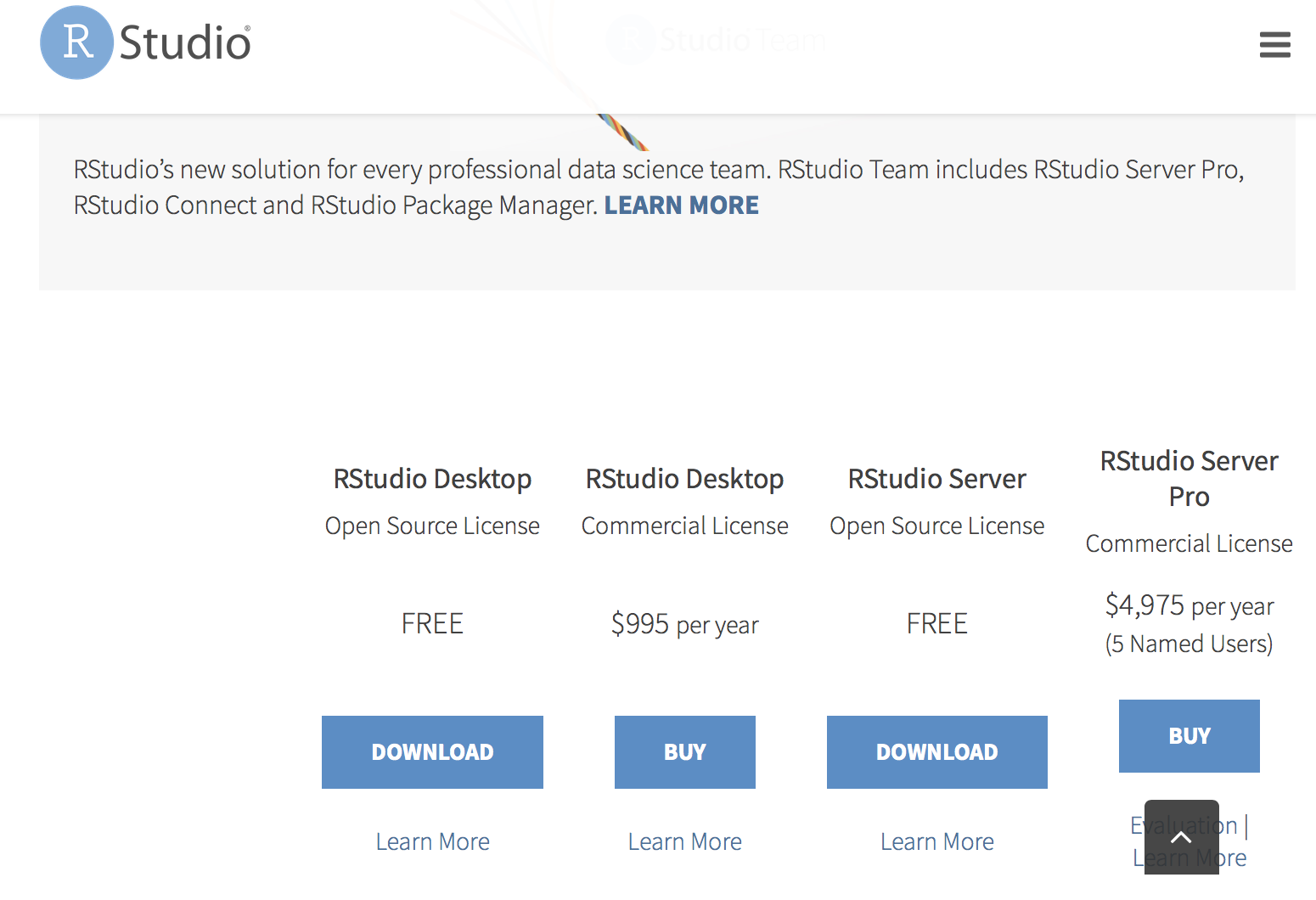
Choose the RStudio Desktop Free option. Once again, an Installer Module should pop up on the computer. Follow its instructions to install RStudio.
Step 3: Open Rstudio and Change The Layout
Open Rstudio by clicking on the RStudio Icon  , and customize it to your liking. When you initially open it, it will look something like this.
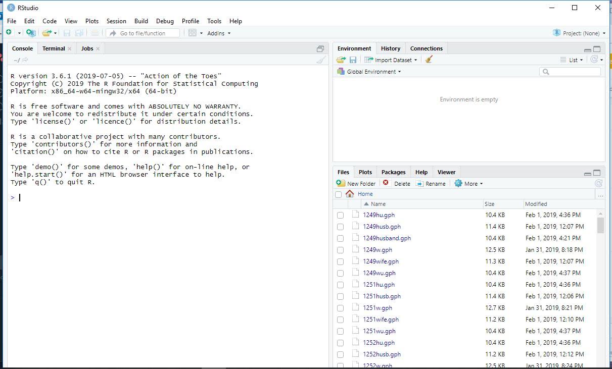 VERY IMPORTANT INFORMATION Right now, there is no section to create scripts. To get a better layout, click on this button on the top right of your screen.
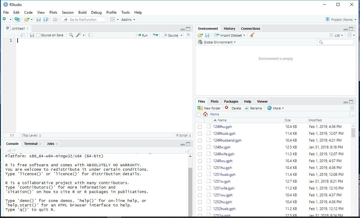
It should now look something like this. The top left box is where scripts are written.

From here, you can play around with the size of each section of the Rstudio interface, and change appearances by clicking on Rstudio->preferences.
Rstudio Layout
Rstudio contains 4 panes: source, console, environment/history/connections, and files/plots/packages/help/viewer. If you didn’t do so earlier, click on the screen minimizing button on the top right of the console pane. Your Rstudio layout should look similar to this.
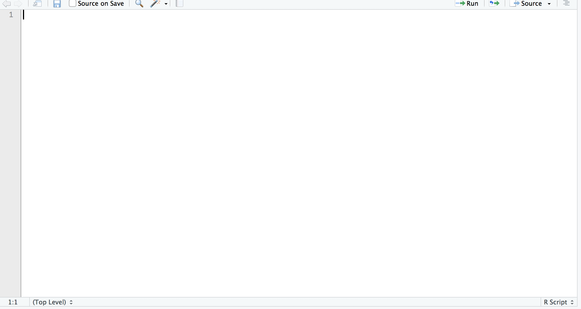
- source is where you write programs in Rstudio. This is similar to a do-file editor in Stata. For any kind of work that will be used for more than just a one time observation, you want to use the source screen.
- console is a place for directly running code This is similar to what you use when opening the Stata application directly. It is only useful for single commands, like installing a package, not for more complicated programs.

- environment/history/connections The environemnt tab of this pane shows you what objects are loaded in R, and allows you to view them

- files/plots/packages/help/viewer Has tabs showing different aspects of your R session. THe most important is help, which can be useful for looking up what new commands do and how to use them.
Running code
There are a few different ways to run R code. The first is to simply type it into your console and enter. Most of your coding, however, should be done in the source pane. To run the entire source file, click on ‘run’ in the upper-right screen of the source pane, and then click ‘run all’. To run a selct few lines, highlight them and click ‘run’ and then ‘run selected lines’.
For convenience, you can also highlight selected lines and then enter command and enter simultaneously on your keyboard.
Packages
Packages are programs written by R users that contain useful functions. Using packages is essential, as while base R (the available R functions that don’t require any packages) has plenty of useful tools, most scripts will require the use of one or more packages. Using a package (in this example, tidyverse) involves the following two commands:
Important: This is the first part of the tutorial in which code is being used. Make sure that you read the comments in the code, as they contain important information. For example, without reading the comment in the code below, you will not be able to run the commands.
Also, sometimes an explanation won’t make total sense at first. That is OK! Try running the code from the tutorial and see what happens. Then, try running it in a slightly different way. If it still doesn’t make sense, it is ok to move on. Many of the techniques will be repeated throughout this tutorial, so you will figure it out eventually.
#Hashtags (#) are used as comments in R. I include the # here because install.packages only needs to be used once. When you run install.packages, make sure to get rid of the #, or it will be treated as a comment and won't work..
#install.packages("tidyverse")
library(tidyverse)
When you install tidyverse, or any other package, a console prompt may ask if it is ok to include files from other sourecs. These will always be safe and are necessary for running a package, so enter ‘yes’ in the console.
You only need to run the install.packages once, but library must be run for each new R session
For now, I will include only tidyverse and ggplot2, as those will be used throughout this document. However, there are a vast number of packages that will be useful for a host of different tasks.
#install.packages("ggplot2")
library(ggplot2)
Possible errors
- You must have the package name in quotes in ‘install.packages’
- You can’t have the package name in quotes in ‘library’
- You must not have a # before install.packages, as that makes it a comment (it is intentionally commented out in this tutorial’s code)
- If you get an error that says “there is no package called ggplot/tidyverse”, that means that install.packages wasn’t successful
Importing and exporting data
This is another ‘setup’ area that can be one of the biggest roadblocks for new users. Be persistent; after this it gets easier. We will try to anticipate possible errors.
Importing
The way you import data depends on on the file type you use. Just like Stata, you have to access the correct filepath on your computer. For this tutorial, please download the files 1. tutorial.csv 2. tutorial.dta. You can go about this either by first changing your directory to the folder like so: Unlike in Stata, you don’t only import the data, but name the data. This is because R can have multiple datasets at once.
#the exact filepath will be unique to each user
setwd("/Users/R")
#<- is (mostly) equivalent to = in R. <- is considered more stylish.#read_csv is a command from the tidyverse package. There is also a base R command called read.csv.
tutorial <- read_csv("tutorial.csv")
or by including the entire filepath in the csv command like so:
tutorial <- read_csv("/Users/R/tutorial.csv")
There are a variety of other commands for downloading other filetypes. The pattern is always the same, along the lines of read_command(filepath), where read_command varies. Sometimes, you will need to use a package in order to read a certain type of file. A useful example is reading Stata13 files. There is also a file in this folder called ‘tutorial.dta’.
#readstata13 must be installed to read stata13 files.
#install.packages("readstata13")
library(readstata13)
tutorial <- read.dta13("/Users/R/tutorial.dta")
Now, try importing both the csv and Stata data.
Possible errors
If you type the filepath in wrong, it will give the error “cannot change working directory” Make sure that you type in the filepath correctly. To learn your current filepath, enter ‘getwd()’. To learn about which files are in your directory currently, enter ls()
Exporting
Exporting data is quite similar to importing it. You must specify the filepath for your output, and use a specific function to write the file of your choice. This is how I would create a csv file called ‘tutorial.csv’ on my desktop. Unlike Stata, you must specify which dataset is being exported, because R holds multiple datasets.
#The function 'write.csv' takes two inputs: the dataset(in this case, 'tutorial'), and the filepath
write.csv(tutorial, "/Users/Desktop/tutorial.csv")
Now, try exporting the tutorial dataset to a location of your choice on your computer. You should be able to find and open it.
Data Structures and Data Management
Data Structures (Especially useful if you have no coding experience or only in Stata)
In the previous section, R’s ability to hold multiple datasets was discussed. R can actually hold a lot more data than that, but to fully undertstand that we must discuss objects and their different types/structures.
In R, all objects have types. The read_csv command (or any similar command) automatically creates an object with the type ‘dataframe’. Dataframes are n by n stores of value, in which we generally assume the rows are observations and the columns are variables. However, there are a wide number of data types in R. These include:
Vectors Values (The common valuyes are strings(words, characters, etc), integers, True/False, decimal numbers) Lists Functions *Plots and many more. Each data type works differently with different functions.
Each data structure has its own properties. Most fucntions require specific types for specific inputs. This may seem annoying, but is usually intuitive and helpful. For example, it would make a lot of sense to use the ‘as.numeric’ command on a vector (turning each categorical value in the vector into numbers), but you wouldn’t want to use the command on an entire dataset. By having these more specific data types, it can be easier to understand exactly how a function works.
Here is how to work with some of the basic datatypes.
Values
string <- "Hello World"
num <- 1
#You can assign an object to another object, rather than directly assigning it
string2 <- string
#Objects can be reassigned after being initially assigned
string <- "Bye World"
binary <- TRUE
Vectors
#the 'c' function tells R to put the values in commas into a vector
vector_nums <- c(1, 2 ,3)
#it can put different kinds values into vectors
vector_strings <- c("We", "Are", "Coding")
#Vectors can be assigned to other vectors
vector_nums2 <- vector_nums
#Values can be assigned into a vector
one <- 1
two <- 2
three <- 3
vector_nums3 <- c(one, two, three)
#Vectors can be created automatically in many different ways, such as
auto <- c(1:100)
#Vector values can be accessed using indexing. This accesses the 54th element of the vector.
fiftyfour <- auto[54]
Dataframes
#Data Frames are usually imported, not created. However, dataframes can be copied:
tutorial2 <- tutorial
#or created using 'data.frame'.
vector_nums <- c(1, 2 ,3)
vector_strings <- c("We", "Are", "Coding")
dataframe_ex1 <- data.frame(vector_strings, vector_nums)
#to access a certain variable in a dataframe, use $
id_vect <- tutorial$ID
Data Management And Variables
As you can see, R can hold many different kinds of data at the same time. This can be extremely useful, as it allows you to create many different objects that can used later on. Sometimes this can be used similarly to how you would use a Stata local.
mypath <- "/Users/jakerothschild"
setwd(mypath)
However, there are also some uses that are different from stata. For example, it might be useful to do something like
id_vect <- tutorial$id
#absolute value
id_vect = abs(id_vect)
It can also be quite useful to have multiple dataframes. Imagine that some analyses need to be run on the entire sample, and some need to be run only on women. I can create a dataframe with only women, and work on both that dataframe and my full sample at the same time. You can avoid constantly saving and reloading data, and only save your underlying data to dropbox.
#Don't worry about the syntax used to create the 'women' dataset yet; what is important is that it is possible to do so.
women <- tutorial %>%
filter(gender == "F")
Tidyverse Basics
Piping
Tidyverse has a very particular syntactic scheme, allowing for avoiding repetition. It uses piping, which allows you to carry through data from one command to the next. Piping will be used throughout the rest of the tutorial. The piping syntax is %>%. Piping essentially means ‘use the object that I used in the previous line’. So, if I write
tutorial %>% any_function()
The function I write in the second line applies to tutorial because I included ‘%>%’.
Here are some examples of how R syntax changes when you use piping. Don’t worry if piping isn’t clear at first; as you work through more examples it will make more sense. Just consider which code is easier to look at and understand.
Also, we use a few different functions in this section to demonstrate piping. These functions will all be explained later; you don’t need to learn them yet.
Without Piping
#creating a copy of tutorial to not mess up our original data
tutorial_copy <- tutorial
#we have to say which dataset we are working with in the mutate command
tutorial_copy <- mutate(tutorial_copy, id_squared = id^2)
With Piping
#Piping allows us to 'pass in' the tutorial dataset and work with it
tutorial_copy <- tutorial %>%
mutate(id_squared = id^2)
#as a result, the mutate command is now automatically working with tutorial.
Advanced piping
Piping may not seem particularly useful in the previous example. However, it can be quite useful for more complicated processes. Don’t worry about understanding the exact functions used below yet.
Example without piping
#creating a copy of tutorial to preserve original dataset
tutorial_copy <- tutorial
#creating new variables
tutorial_copy <- mutate(tutorial_copy, score_squared = score^2)
tutorial_copy <- mutate(tutorial_copy, score_squared_bucket = ifelse(score_squared < 100, 0, 1))
#creating a grouped dataset
tutorial_groups <- group_by(tutorial_copy, score_squared_bucket)
#summarizing the grouped dataset
tutorial_summary <- summarize(tutorial_groups, avg_score = mean(score_squared))
Example with piping
#we start by saying that our new dataset, tutorial summary is equal to tutorial
tutorial_summary <- tutorial %>%
#but by piping, we tell r that we are still working with the tutorial dataset
#so we don't need to include tutorial in our commands again
mutate(score_squared = score^2) %>%
mutate(score_squared_bucket = ifelse(score_squared< 100, 0, 1)) %>%
#here, we group by a certain variable (this is equivalent to bysort in stata)
group_by(score_squared_bucket) %>%
#now, because of piping, we are working with the grouped version of the dataset.
summarize(avg_score = mean(score_squared))
As you can see, piping allows us to use less keystrokes, create less datasets, and (although it may not seem it at first) create clearer code.
Data Cleaning
The vast majority of cleaning operations can be done using a few simple commands.
Observing Data
There are two ways to observe datasets (or other data, like vectors). The first is to click on data in the Global Environment tab. That can be annoying if you have many datasets stored, so the second option is the view function. Its syntax is simple
view(tutorial)
Sorting
Sorting is useful both for viewing data, and for certain cleaning functions. The tidyverse function for sort is arrange. The function requires a dataset, and condition(s) for sorting. In this example, we pipe in the dataset(as we will do for most future examples)
tutorial_copy <- tutorial
#one condition
tutorial_copy <- tutorial %>%
arrange(score)
##two conditions
tutorial_copy <- tutorial
tutorial_copy <- tutorial %>%
arrange(gender, score)
##Can do opposite order using 'desc'
tutorial_copy <- tutorial
tutorial_copy <- tutorial %>%
arrange(desc(score))
Removing observations
The basic tidyverse method for removing observations is the filter function Filter only keeps observations where the condition is met for that variable.
Basic Conditions
#creating a copy to not change original dataset
tutorial_copy <- tutorial
#piping is used to work within the tutorial dataset
tutorial_copy <- tutorial_copy %>%
#only keeping observations where gender is equal to "F"
filter(gender == "F")
Logical statements can be used for more complicated filters ###More conditions
#creating a copy to not change original dataset
tutorial_copy <- tutorial
#piping is used to work within the tutorial dataset
tutorial_copy <- tutorial_copy %>%
#only keeping observations where gender is equal to M or F
filter(gender == "F"|gender == "M")
#restoring tutorial copy
tutorial_copy <- tutorial
#piping is used to work within the tutorial dataset
tutorial_copy <- tutorial_copy %>%
#only keeping observations where gender doesn't equal F
filter(gender != "F")
Removing variables from dataset
To choose variables to keep, we use the select function
tutorial_copy <- tutorial
tutorial_copy <- tutorial_copy %>%
select(gender, score)
To remove variables, use the identical function but with ‘-’ before variables we wish to remove
tutorial_copy <- tutorial
tutorial_copy <- tutorial_copy %>%
select(-gender, -score)
New Variables
To create new variables, use the mutate function. Multiple variables can be created at once with this function.
tutorial_copy <- tutorial
#just one variable
tutorial_copy <- tutorial_copy %>%
mutate(score_x_2 = score * 2)
##multiple
tutorial_copy <- tutorial_copy %>%
mutate(score_x_4 = score * 4,
score_x_3 = score * 3)
ifelse is a very useful function for creating categorical variables. It takes three arguments: a condition and two outcomes. It then assigns variables to the first outcome if it meets the condition, and to the second outcome if not.
tutorial_copy <- tutorial
#this function creates the variable score_greaterthan_10. This variable is equal to 1 if score is > 10, and 0 if score < 10
tutorial_copy <- tutorial_copy %>%
mutate(score_greaterthan_10 = ifelse(score > 10, 1 , 0))
Nested ifelse statements can create more than two buckets. There are some other functions that can do this more efficiently, depending on the specific task, but that is beyond the scope of this tutorial.
tutorial_copy <- tutorial
tutorial_copy <- tutorial_copy %>%
#The first ifelse states that if score is <10, score_buckets should be equal to 0, but if score is > 10, we should go into a second ifelse statement.
mutate(score_buckets = ifelse(score < 10, 0 ,
ifelse(score >= 10 & score < 20, 1, 2)))
#the second ifelse only is read if the first ifelse condition isn't met. It tells us that we should set score_buckets to 1 if score is between 10 and 20, and 2 otherwise.
Renaming Variables
Renaming variables is simple. Use the rename function
tutorial_copy <- tutorial
tutorial_copy <- tutorial_copy %>%
rename(identification = id)
Reshaping
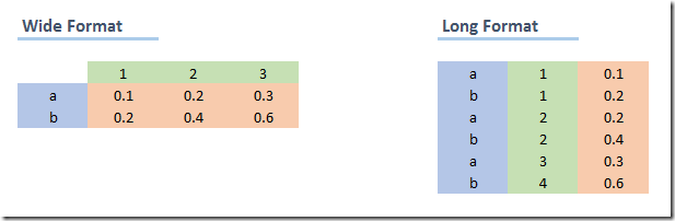
Sometimes, it will be important to change the format of your data from wide to long or long to wide. A long dataset changes the unit of analysis such that each row contains less data, and as a result, there are more rows. This example should show the difference.
Note that both datasets show the exact same information. However, it is usually easier to work with one type of data, depending on the task at hand.
(a) Wide to long
Gather is used to reshape data from wide to long. This transformation tends to be more common. Currently, each row contains two scores: score and score2. When we reshape the data to long, we will have create a new variable, ‘round’, that tells us which type of score the data is. So, each row will only contain one score instead of two, which means that then number of rows will double.
The gather function takes 4 arguments; 1)The dataset, which in this case is piped 2)A key string, which is the name of the column used to distinguish between the different types of values 3)A value string, which is the name of the column of the combined outcome variable, in this case score 4)A vector, which contains the columns that should be combined into 1, in this case score
tutorial_long <- tutorial %>%
gather("score_type", "score", c(score, score2))
While in this example we use only a single column, gather can be used for multiple columns. Gather isn’t the easiest command to use, so make sure you know exactly what you want your data to look like before using it.
(b) Long to wide
Spread is the function used to reshape data from long to wide. In the tutorial_long dataset, there should now be 12 observations of the dataset. We will shift it back to its original form using spread.
Spread takes three arguments: 1)The dataset, which in this case is piped 2)A key, which is the variable in the dataset that describes which type of data it is. In this case, it is score_type, as it distinguishes between score and score2 3)A value, which is the variable that contains the information, which in this case is score.
tutorial_wide <- tutorial_long %>%
spread(score_type, score)
Now, each row contains two observations, one of each score type. Similarly to gather, this commmand can be tricky to use, and you must have a clear understanding of your data.
Missing Values
In R, is.na(variable) evaluates to true if the variable is missing. !is.na(variable) does the opposite.
tutorial_copy <- tutorial
tutorial_copy <- tutorial_copy %>%
mutate(missing_id = is.na(id))
tutorial_copy <- tutorial_copy %>%
mutate(non_missing_id = !is.na(id))
Datasets: Altering or Creating New
In all of these examples, I have been creating a copy of my dataset and then changing that copy. That is unnecessary in R. For example, to create a tutorial_copy dataset with a missing_id variable, I can simply do:
tutorial_copy <- tutorial %>%
mutate(missing_id = is.na(id))
However, I could also simply adjust my original tutorial dataset. While the ability to hold multiple datasets at once is a convenient feature of R, that doesn’t mean you want to create a new dataset with every single change. It is up to the user to figure out how to create protocols for when to create a new dataset, and when to adjust an old one.
Summary statistics
R has somewhat more challenging syntax than Stata for summary statistics, but also allows for a greater level of customization in choice of summary statistics. You can also easily create and work with summary statistic datasets, which tends to be a poor opton in Stata.
Summarize
Summarize is the main tidyverse tool for both looking at summary statistics and creating summary datasets. Like other tidyverse commands, it works best with piping. A variety of statistics, such as mean, minmax, number of observations, standard deviation, and more can be calculated this way.
#First create a dataset without null values, or summarize returns NA
tutorial_no_NA <- tutorial %>%
filter(!is.na(score))
##We can create one specific summary statisitcs
tutorial_no_NA %>%
summarize(avg_score = mean(score))
##   avg_score
## 1      25.9
##Or multiple
tutorial_no_NA %>%
summarize(avg_score = mean(score), sd_score = sd(score))
##   avg_score sd_score
## 1      25.9 15.82157
##We can use filter to summarize conditionally
tutorial_no_NA %>%
filter(score > 5) %>%
summarize(avg_score = mean(score), sd_score = sd(score))
##   avg_score sd_score
## 1  28.66667 13.98213
##We can create a dataset of summary statistics
tutorial_summary <- tutorial_no_NA %>%
summarize(avg_score = mean(score), sd_score = sd(score))
group_by
The ‘group_by’ function is similar to Stata’s ‘by’ command. It splits data into a bunch of smaller chunks, and then applies the next set of code to each chunk individually. This allows you to get group counts, similar to tab.
##Standard count of gender
tutorial %>%
group_by(gender) %>%
summarize(count = n())
## # A tibble: 2 x 2
##   gender count
##
## 1 F          5
## 2 M          6
##Can do multiple groups
tutorial %>%
group_by(gender, position) %>%
summarize(count = n())
## # A tibble: 4 x 3
## # Groups:   gender [2]
##   gender position   count
##
## 1 F      Rassistant     2
## 2 F      Rassociate     3
## 3 M      Intern         2
## 4 M      Surveyor       4
##And can filter
tutorial %>%
filter(score > 10) %>%
group_by(gender, position) %>%
summarize(count = n())
## # A tibble: 4 x 3
## # Groups:   gender [2]
##   gender position   count
##
## 1 F      Rassistant     2
## 2 F      Rassociate     3
## 3 M      Intern         1
## 4 M      Surveyor       3
We can go beyond counts and get group means, maxs, etc
##Mean Score By Gender
tutorial %>%
group_by(gender) %>%
summarize(mean = mean(score))
## # A tibble: 2 x 2
##   gender  mean
##
## 1 F       32.4
## 2 M       NA
##With Filtering
tutorial %>%
filter(score > 10) %>%
group_by(gender) %>%
summarize(mean = mean(score))
## # A tibble: 2 x 2
##   gender  mean
##
## 1 F       32.4
## 2 M       24
group_by is useful for creating new summary statistic datasets. Many of the ggplot commands work much better with data in this format
gender_means <- tutorial %>%
group_by(gender) %>%
summarize(mean = mean(score))
Data Visualization
ggplot
ggplot is an R package designed to be a ‘grammar of graphics’. This means that rather than memorizing syntax for a given output, creating ggplots requires thinking about how to map data onto different visual features. This allows for much greater control of graphics and for more logically created graphics. For more information about the philsophy of ggplot, read this - The ggplot command requires two inputs: data and aesthetics, although you will almost always want to include geoms, and often themes, labels, and scaling Through this section, we will iteratively build a beautiful plot.
Aesthetics
Aesthetics describe how your data is being mapped onto a physical plot (what this means may be unclear at first, so hang in there). Every ggplot requires at least one aesthetic, but more can be used.
#aes is short for aesthetics
p <- ggplot(data = tutorial, aes(x = score, y = score2))
p
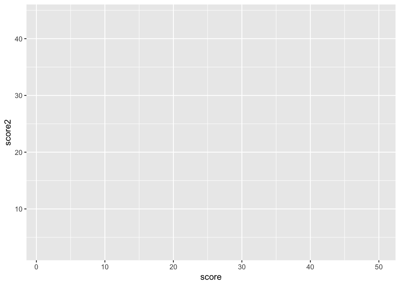
As you can see, the x axis is score, and the y axis is score2. This is what aesthetics does; it takes a variable from the dataset and maps that variable onto a feature of the graph. In this case, we only use two axes, but much more is possible.
Geoms
We currently have an empty graph, which isn’t telling us much of anything. What we now want to do is add a geom, which are different kinds of physical shapes that represent the data that has been mapped to aesthetics.
#to add features to a ggplot, we use +
p <- p + geom_point()
p

You can use different kinds of geoms, still using the same aesthetics
#resetting p
p <- ggplot(data = tutorial, aes(x = score, y = score2))
#don't worry about the syntax, but this adds a regression line
p <- p + geom_smooth(method = 'lm',se = F)
p

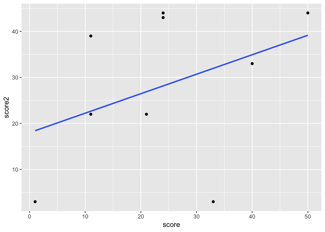
You can, and often should use multiple geoms on the same graph
#don't worry about the syntax, but this adds a regression line
p <- p + geom_point()
p
There are also some aesthetics that work best with geoms. For example, now we can add in gender as a third aesthetic, and map it to color
p <- ggplot(data = tutorial, aes(x = score, y = score2, color = gender)) +
geom_point() +
geom_smooth(method = 'lm', se = F)
p

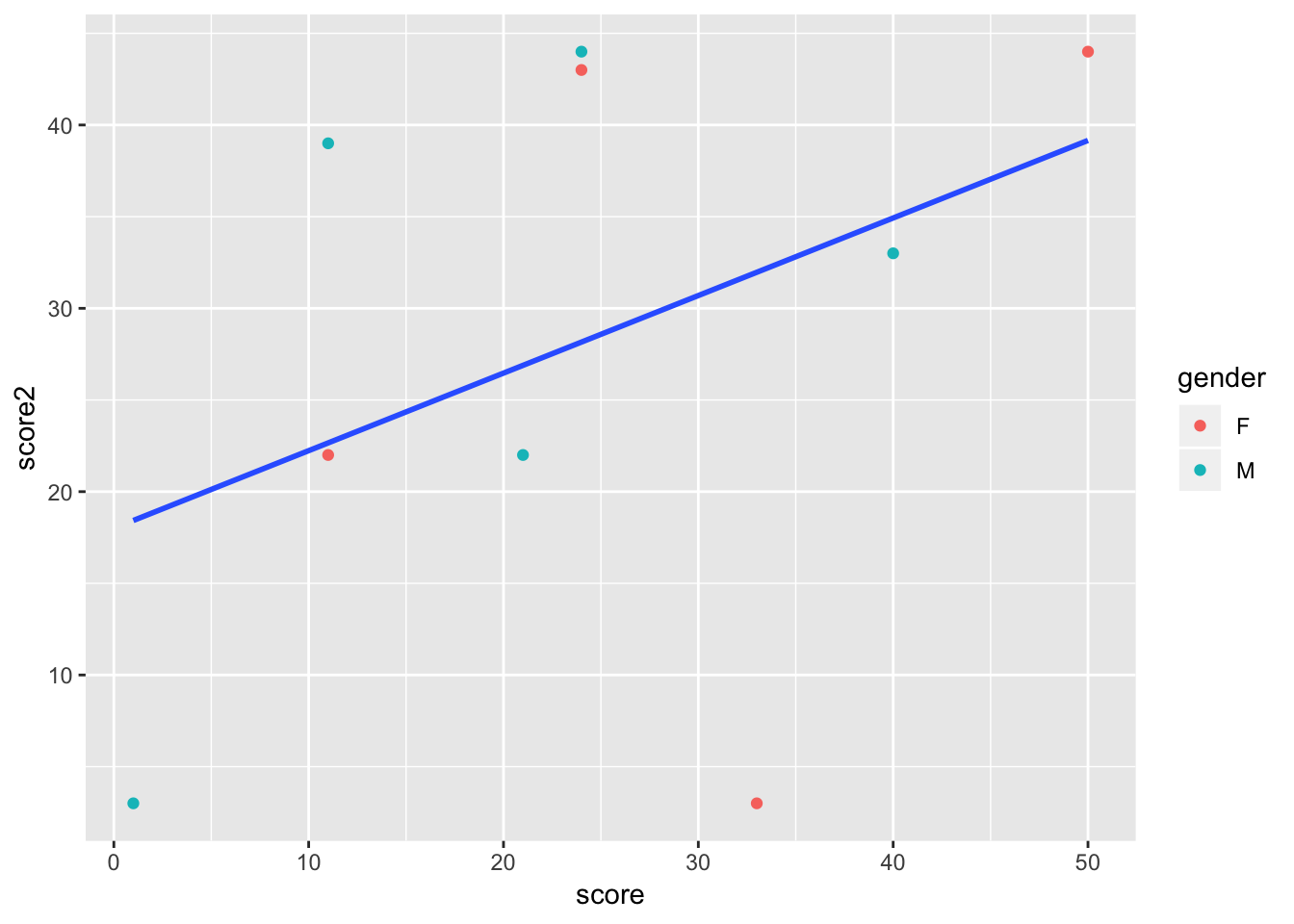
If you want some geoms to have aesthetics but not others, you can use aes in the geom itself, rather than the ggplot function. In this plot, the points are colored by gender, but we only have a single regresion line.
p <- ggplot(data = tutorial, aes(x = score, y = score2)) +
geom_point(aes(color = gender)) +
geom_smooth(method = 'lm', se = F)
p
As you can see, with just the basic structure of aesthetics and geoms, you can build more and more complex plots. You are also able to build iteratively, as you can start with single aesthetics and geoms, and add and take away features until your data is shown most clearly.
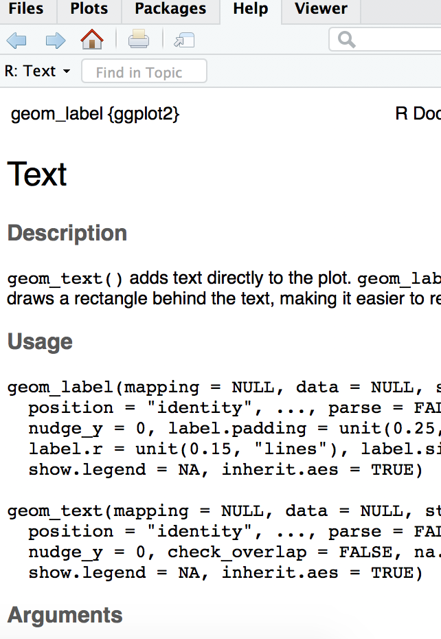
Some common geoms are: * geom_point (points for scatterplots) * geom_smooth (estimate lines, can be linear or nonlinear) * geom_bar (bar charts) * geom_density (density plots) * geom_histogram (histograms) * geom_abline (unfitted lines, for example to show what a linear relationship would look like) * geom_errorbar (error bars) * geom_text (for labeling bar chart estimates, for example)
Scales
By default, ggplot scales the graph to the data, so p is scaled from 0-50 on the x axis, and 0-40 on the y axis. If we assume that score and score2 are similar in nature, we would want them to be scaled identically, or we may mislead the audience. To do this, we use the function scale_AESTHETIC_SCALING, where in this case AESTHETIC is y, and SCALING is continous.
p <- p + scale_y_continuous(limits = c(0, 50))
p

Any aesthetic can be changed using the scale command, and you will have the options of continous, discrete, or manual, depending on the type of data.
Labels and Legends
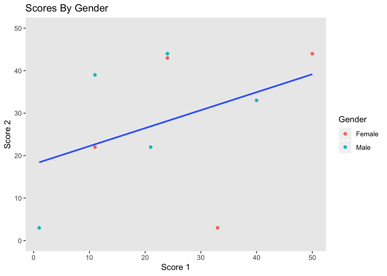
Our graph, p now does depict certain aspects of our data. However, it isn’t very clear what exactly it is showing, as there is no title, and the legend and axis labels are based on the data, and therefore unclear. The main function used for labeling is labs, which can affect the title and any aesthetics.
p <- p + labs(title = "Scores By Gender", x = "Score 1", y = "Score 2", color = "Gender")
p

the legend labels using the scale function from the previous section.
p <- p + scale_color_discrete(labels = c("Female", "Male"))
p

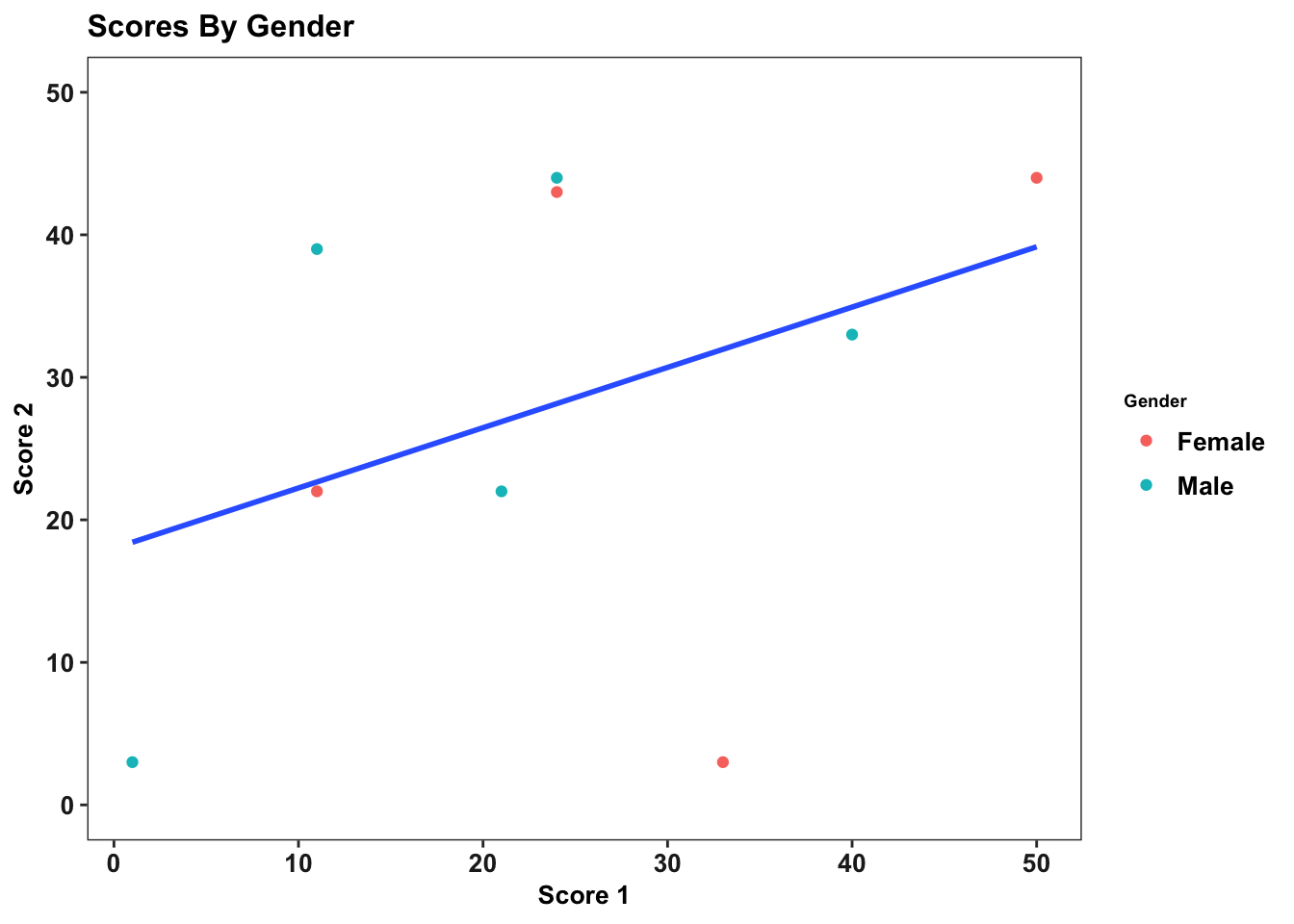
Themes
Now, all that is left to do is make the graph look nicer. To do this, we use the theme command. There are dozens of options that can be used for the theme command, so you will have to figure out for yourself what you think works best. The syntax is straightforward; this is how you would remove the panel grid.
p <- p + theme(panel.grid = element_blank())
p
The best practice is to create a theme and then use it across all charts. This is another situation in which R’s flexibility in storing objects is very useful. For example, we can create a theme like so.
my_theme <- theme_bw() +
theme(text = element_text(size = 10, face = "bold", color = "black"),panel.grid = element_blank(),axis.text = element_text(size = 10, color = "gray13"), axis.title = element_text(size = 10, color = "black"), legend.text = element_text(colour="Black", size=10), legend.title = element_text(colour="Black", size=7), plot.subtitle = element_text(size=14, face="italic", color="black"))
And then use it for not only this graph, but all later graphs
p <- p + my_theme
p
It is even possible to have your theme be a function, which allows you to customize your theme for different situations, but that is a more advanced topic and unneccessary for creating excellent ggplots.
Data Types
One thing that may happen to you as you try creating ggplots is that you sometimes have hard-to-understand errors or create useless graphs. For example,
bad <- ggplot(data = tutorial, aes(x = gender)) + geom_density()
bad
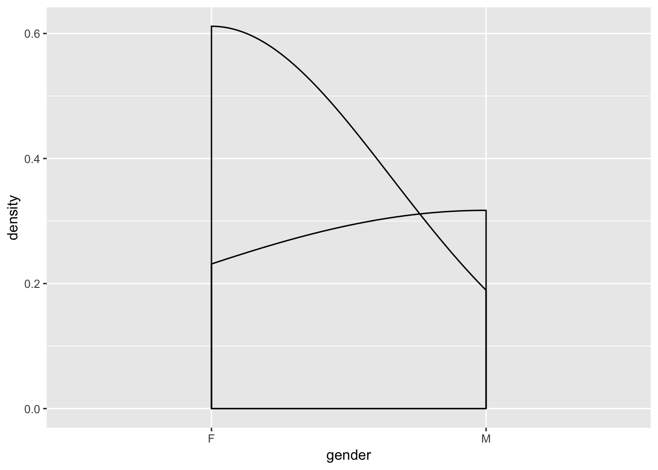
is entirely meaningless,while
#error <- ggplot(data = tutorial, aes(x = gender)) + geom_bar(stat = 'identity')
#error
gives you an error, even though the syntax is accurate (commented out to avoid having the file crash). This is because certain plots only work with certain kinds of data. For example, a bar chart will work best with one continuous variable and one categorical variable. Scatterplots work well with two continuous variables. Whether a misuse of a variable results in an error or a bad graph depends on the specific type of error, but either way, you need to understand your data before trying to visualizate it.
Advanced ggplot
Once you have gotten comfortable with ggplot, there are some more complicated packages that can be used alongside ggplot to create some more advanced graphics.
Examples and more info
Here are some articles that have more examples of ggplot syntax and technique, along with some more information about the package.
Regressions
Basic Regressions
A standard linear regression uses the command lm takes two arguments: A formula and data. The syntax works as follows
reg <- tutorial %>%
#score is the dependent variable, score2 is the independent variable. Our formula is score = B(score2) + error
#data = , is used because we pass in the tutorial dataset using piping
lm(score ~ score2, data = .)
We can use multiple independent variables/controls using the same syntax, with + separating different regression inputs in the formula.
reg_gend <- tutorial %>%
#In this case, our formula is score = B1(score2) + B2(gender) + error
lm(score ~ score2 + gender, data = .)
And we can measure interaction effects using * in our formula.
reg_gend_interation <- tutorial %>%
lm(score ~ score2 + gender + score2*gender, data = .)
Output
You may have noticed that there hasn’t been an output from the previous regressions. This is because all we did is create the regression object (which happpens to be a list). There are a few ways to see regression results.
The easiest of these is summary. When using regressions for
summary(reg)
##
## Call:
## lm(formula = score ~ score2, data = .)
##
## Residuals:
##     Min      1Q  Median      3Q     Max
## -16.835 -10.674  -5.285  14.339  20.352
##
## Coefficients:
##             Estimate Std. Error t value Pr(>|t|)
## (Intercept)  13.7007    10.3570   1.323    0.227
## score2        0.3624     0.3219   1.126    0.297
##
## Residual standard error: 15.12 on 7 degrees of freedom
##   (2 observations deleted due to missingness)
## Multiple R-squared:  0.1533, Adjusted R-squared:  0.03237
## F-statistic: 1.268 on 1 and 7 DF,  p-value: 0.2973
tutorial %>%
lm(score ~ score2 + gender + score2*gender, data = .) %>%
summary
##
## Call:
## lm(formula = score ~ score2 + gender + score2 * gender, data = .)
##
## Residuals:
##       1       2       3       4       5       6       8       9      11
##   4.719   9.389  -5.724  16.731 -13.833  18.186 -17.087  -3.348  -9.033
##
## Coefficients:
##                Estimate Std. Error t value Pr(>|t|)
## (Intercept)     22.9046    15.7829   1.451    0.206
## score2           0.2356     0.4826   0.488    0.646
## genderM        -17.6895    22.3902  -0.790    0.465
## score2:genderM   0.2675     0.6951   0.385    0.716
##
## Residual standard error: 16.31 on 5 degrees of freedom
##   (2 observations deleted due to missingness)
## Multiple R-squared:  0.2959, Adjusted R-squared:  -0.1265
## F-statistic: 0.7005 on 3 and 5 DF,  p-value: 0.591
When we create a regression and store it as an object, we have created a list that contains tables. When including regression output in a report, using a table display package such as kableExtra is the best method of outputting the results. The syntax is somewhat complicated, so it will not be included in this document. A quick internet search will provide examples and guides like this one.
Other regressions
Other regressions usually require a package, but use the same syntax as lm. For example, for a fixed effects regression, one must install the lfe package, and use a similar command to above, but with ‘felm’ replacing ‘lm’. For a logistic regression, the glm package is required, and ‘glm’ replaces ‘lm’ in the above commands. There are more regression types and packages than can be employed for the circumstance.
Functional progamming
It is not necessary to use a functional programming to use R and Tidyverse effectivelty, especially for smaller tasks. In fact, we recommend that you learn the basics of R before switching to a functional style of programming, as you will need to be comfortable with R and its syntax. However, once you gain some experience, functions are an excellent tool for reducing errors, creating more readable code, taking less time to finish tasks, and debugging more easily. For longer, more complex programs, they are incredibly useful.
What are functions?
Functions are similar to commands in stata – they take in some kind input, and do something based on that input, like create a new dataset or a plot. To code in R is to use functions created by other people. These functions, of course, are designed to be quite general.
What is functional programming?
Functional programming is a method of programming in which a script with a large, complicated goal (like cleaning a dataset) is broken up into smaller, more modular, hopefully repeatable tasks. For each smaller task, you create a user-defined function, designed for your specific task. Your main script will then run only a few lines of code, where each line is a function you have created. Each function can include other, smaller functions, which can be used repeatedly.
Why use functional programming?
The main reason to use functional coding is to avoid repetition. Without functions, when you repeat the same task, you will either have to * create a loop, which can be unfeasible and is often confusing, as well as prone to bugs, OR * copy a paste a lot of code, which is hard to follow, time-consuming, and creates a lot of opportunities for errors.
Functions allow you to do repetitive tasks with minimal amounts of code. For example, imagine that for a group of variables, you want to get rid of missing values, and then use a command to predict the values of for those observations. Rather than continuously using the same 4 lines, you can create a function containing those 4 lines. You can then run that function on each variable. Furthermore, there is a tidyverse function that allows you to do all of this in only one line.
It may not seem like a big deal when the function is only 4 lines of code; why not just repeat it a few times. However, when tasks get more complicated, repeating them over and over can be massively inefficient; retyping 100 lines of code for 12 variables with slightly different syntax is not how you want to spend your time coding, and is also very difficult for another user to follow.
Syntax
Functions, like many other aspects of R, are stored as objects in R. Imagine I want to create a simple function called replace_missing_with_number, which as the name suggests, takes the missing values in a vector and replaces them with a number. I label replace_missing_with number, and include three things in each function:
- 0, 1, or multiple inputs, that will be used in the function body
- A function body, which can include commands, other function calls, and more
- A return statement, which is the output of the function
#we define replace_missing_with_number as a function requiring two inputs: a variable and a number
#the function won't work unless variable is a vector and number is an integer
replace_missing_with_number <- function(variable, number) {
#the function body is included between { and }. In this case, it is only two lines, but functions can be 10s or 1000s of lines long
variable <- ifelse(is.na(variable), number, variable)
#At the end, a return command is neccessary to denote the function's output.
return(variable)
}
Now that the function has been defined, it can be used at any time
score <- tutorial$score
id <- tutorial$id
#it works as promised with a vector
score <- replace_missing_with_number(score, 0)
#and can be reused
id <- replace_missing_with_number(id, 999)
#it does nothing with a dataframe
tutorial_copy <- replace_missing_with_number(tutorial, 0)
Apply
The apply family of functions is one of the most convenient features of R, and a great reason to use a functional style of programming. The three most basic commands – apply, lapply, and sapply – allow you to repeat a function over a matrix, list, or vector. This means that by creating a function and running one or two commands, you can apply a cleaning function to an entire dataset, without using any for loops!
The apply function is somewhat advanced, so this tutorial will only show an example of the sapply function. Here is an intraductory explanation, while here is a more advanced and complete explanation of all of the apply functions.
In this example, we will apply our replace_missing_with_number function to each row of our dataset. It only takes two lines(that could be condensed to one, which is much easier than a for loop)
Examples
This link discusses the reason for using functional programming in greater detail, and includes some more complicated functions.
R Markdown
This document was created entirely in R Markdown, R’s document creating tool. Using R Markdown is incredibly simple and straightforward. In the Rstudio interface, click on File -> New File -> R Markdown. It will open up a tab in which you can input the author, title, and output (these can all be changed later). After clicking OK, a new tab will appear. It should look something like this
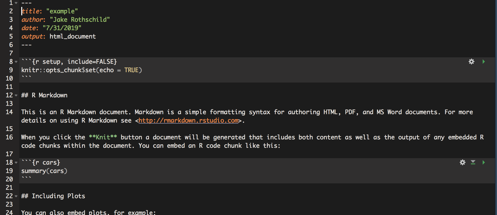
The way R Markdown works is that it doesn’t treat text as code unless specifically instructed too. So, if you write a command like read_csv(filepath), and then try to run it, nothing will happen. To create R code, use the following structure
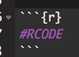
This way, you can switch back and forth between plain text like this
print("and code like this")
## [1] "and code like this"
When you want to see the output of your RMD script, you click the knit button on the Rstudio interface. You can then choose to knit to html, word, or pdf. There is no cost of knitting, so I suggest you knit early and often to make sure that everything is working.
Once you have a document you like, there are various publishing options. Most only work with html, which tends to be the most compatible with R Markdown in general.
There are also a variety of advanced options for R Markdowns. These include creating a table of contents, putting different outputs into tabs to reduce the length of your report, hiding code so reports only show output and text, and a host of text formatting tools.
Cheat sheet of useful functions
This is not a complete list. To do other things, you will often need to google, but R is quite well-documented.
Installing packages
The basic tidyverse method for removing observations is the filter function Filter only keeps observations where the condition is met for that variable.
Basic Conditions
#creating a copy to not change original dataset
tutorial_copy <- tutorial
#piping is used to work within the tutorial dataset
tutorial_copy <- tutorial_copy %>%
#only keeping observations where gender is equal to "F"
filter(gender == "F")
Logical statements can be used for more complicated filters ###More conditions
#creating a copy to not change original dataset
tutorial_copy <- tutorial
#piping is used to work within the tutorial dataset
tutorial_copy <- tutorial_copy %>%
#only keeping observations where gender is equal to M or F
filter(gender == "F"|gender == "M")
#restoring tutorial copy
tutorial_copy <- tutorial
#piping is used to work within the tutorial dataset
tutorial_copy <- tutorial_copy %>%
#only keeping observations where gender doesn't equal F
filter(gender != "F")
Removing variables from dataset
To choose variables to keep, we use the select function
tutorial_copy <- tutorial
tutorial_copy <- tutorial_copy %>%
select(gender, score)
To remove variables, use the identical function but with ‘-’ before variables we wish to remove
tutorial_copy <- tutorial
tutorial_copy <- tutorial_copy %>%
select(-gender, -score)
New Variables
To create new variables, use the mutate function. Multiple variables can be created at once with this function.
tutorial_copy <- tutorial
#just one variable
tutorial_copy <- tutorial_copy %>%
mutate(score_x_2 = score * 2)
##multiple
tutorial_copy <- tutorial_copy %>%
mutate(score_x_4 = score * 4,
score_x_3 = score * 3)
ifelse is a very useful function for creating categorical variables. It takes three arguments: a condition and two outcomes. It then assigns variables to the first outcome if it meets the condition, and to the second outcome if not.
tutorial_copy <- tutorial
#this function creates the variable score_greaterthan_10. This variable is equal to 1 if score is > 10, and 0 if score < 10
tutorial_copy <- tutorial_copy %>%
mutate(score_greaterthan_10 = ifelse(score > 10, 1 , 0))
Nested ifelse statements can create more than two buckets. There are some other functions that can do this more efficiently, depending on the specific task, but that is beyond the scope of this tutorial.
tutorial_copy <- tutorial
tutorial_copy <- tutorial_copy %>%
#The first ifelse states that if score is <10, score_buckets should be equal to 0, but if score is > 10, we should go into a second ifelse statement.
mutate(score_buckets = ifelse(score < 10, 0 ,
ifelse(score >= 10 & score < 20, 1, 2)))
#the second ifelse only is read if the first ifelse condition isn't met. It tells us that we should set score_buckets to 1 if score is between 10 and 20, and 2 otherwise.
Renaming Variables
Renaming variables is simple. Use the rename function
tutorial_copy <- tutorial
tutorial_copy <- tutorial_copy %>%
rename(identification = id)
Reshaping
Sometimes, it will be important to change the format of your data from wide to long or long to wide. A long dataset changes the unit of analysis such that each row contains less data, and as a result, there are more rows. This example should show the difference.
Note that both datasets show the exact same information. However, it is usually easier to work with one type of data, depending on the task at hand.
(a) Wide to long
Gather is used to reshape data from wide to long. This transformation tends to be more common. Currently, each row contains two scores: score and score2. When we reshape the data to long, we will have create a new variable, ‘round’, that tells us which type of score the data is. So, each row will only contain one score instead of two, which means that then number of rows will double.
The gather function takes 4 arguments; 1)The dataset, which in this case is piped 2)A key string, which is the name of the column used to distinguish between the different types of values 3)A value string, which is the name of the column of the combined outcome variable, in this case score 4)A vector, which contains the columns that should be combined into 1, in this case score
tutorial_long <- tutorial %>%
gather("score_type", "score", c(score, score2))
While in this example we use only a single column, gather can be used for multiple columns. Gather isn’t the easiest command to use, so make sure you know exactly what you want your data to look like before using it.
(b) Long to wide
Spread is the function used to reshape data from long to wide. In the tutorial_long dataset, there should now be 12 observations of the dataset. We will shift it back to its original form using spread.
Spread takes three arguments: 1)The dataset, which in this case is piped 2)A key, which is the variable in the dataset that describes which type of data it is. In this case, it is score_type, as it distinguishes between score and score2 3)A value, which is the variable that contains the information, which in this case is score.
tutorial_wide <- tutorial_long %>%
spread(score_type, score)
Now, each row contains two observations, one of each score type. Similarly to gather, this commmand can be tricky to use, and you must have a clear understanding of your data.
Missing Values
In R, is.na(variable) evaluates to true if the variable is missing. !is.na(variable) does the opposite.
tutorial_copy <- tutorial
tutorial_copy <- tutorial_copy %>%
mutate(missing_id = is.na(id))
tutorial_copy <- tutorial_copy %>%
mutate(non_missing_id = !is.na(id))
Datasets: Altering or Creating New
In all of these examples, I have been creating a copy of my dataset and then changing that copy. That is unnecessary in R. For example, to create a tutorial_copy dataset with a missing_id variable, I can simply do:
tutorial_copy <- tutorial %>%
mutate(missing_id = is.na(id))
However, I could also simply adjust my original tutorial dataset. While the ability to hold multiple datasets at once is a convenient feature of R, that doesn’t mean you want to create a new dataset with every single change. It is up to the user to figure out how to create protocols for when to create a new dataset, and when to adjust an old one.
Summary statistics
R has somewhat more challenging syntax than Stata for summary statistics, but also allows for a greater level of customization in choice of summary statistics. You can also easily create and work with summary statistic datasets, which tends to be a poor opton in Stata.
Summarize
Summarize is the main tidyverse tool for both looking at summary statistics and creating summary datasets. Like other tidyverse commands, it works best with piping. A variety of statistics, such as mean, minmax, number of observations, standard deviation, and more can be calculated this way.
#First create a dataset without null values, or summarize returns NA
tutorial_no_NA <- tutorial %>%
filter(!is.na(score))
##We can create one specific summary statisitcs
tutorial_no_NA %>%
summarize(avg_score = mean(score))
## avg_score ## 1 25.9
##Or multiple
tutorial_no_NA %>%
summarize(avg_score = mean(score), sd_score = sd(score))
## avg_score sd_score ## 1 25.9 15.82157
##We can use filter to summarize conditionally
tutorial_no_NA %>%
filter(score > 5) %>%
summarize(avg_score = mean(score), sd_score = sd(score))
## avg_score sd_score ## 1 28.66667 13.98213
##We can create a dataset of summary statistics
tutorial_summary <- tutorial_no_NA %>%
summarize(avg_score = mean(score), sd_score = sd(score))
group_by
The ‘group_by’ function is similar to Stata’s ‘by’ command. It splits data into a bunch of smaller chunks, and then applies the next set of code to each chunk individually. This allows you to get group counts, similar to tab.
##Standard count of gender
tutorial %>%
group_by(gender) %>%
summarize(count = n())
## # A tibble: 2 x 2 ## gender count ## ## 1 F 5 ## 2 M 6
##Can do multiple groups
tutorial %>%
group_by(gender, position) %>%
summarize(count = n())
## # A tibble: 4 x 3 ## # Groups: gender [2] ## gender position count ## ## 1 F Rassistant 2 ## 2 F Rassociate 3 ## 3 M Intern 2 ## 4 M Surveyor 4
##And can filter
tutorial %>%
filter(score > 10) %>%
group_by(gender, position) %>%
summarize(count = n())
## # A tibble: 4 x 3 ## # Groups: gender [2] ## gender position count ## ## 1 F Rassistant 2 ## 2 F Rassociate 3 ## 3 M Intern 1 ## 4 M Surveyor 3
We can go beyond counts and get group means, maxs, etc
##Mean Score By Gender
tutorial %>%
group_by(gender) %>%
summarize(mean = mean(score))
## # A tibble: 2 x 2 ## gender mean ## ## 1 F 32.4 ## 2 M NA
##With Filtering
tutorial %>%
filter(score > 10) %>%
group_by(gender) %>%
summarize(mean = mean(score))
## # A tibble: 2 x 2 ## gender mean ## ## 1 F 32.4 ## 2 M 24
group_by is useful for creating new summary statistic datasets. Many of the ggplot commands work much better with data in this format
gender_means <- tutorial %>%
group_by(gender) %>%
summarize(mean = mean(score))
Data Visualization
ggplot
ggplot is an R package designed to be a ‘grammar of graphics’. This means that rather than memorizing syntax for a given output, creating ggplots requires thinking about how to map data onto different visual features. This allows for much greater control of graphics and for more logically created graphics. For more information about the philsophy of ggplot, read this - The ggplot command requires two inputs: data and aesthetics, although you will almost always want to include geoms, and often themes, labels, and scaling Through this section, we will iteratively build a beautiful plot.
Aesthetics
Aesthetics describe how your data is being mapped onto a physical plot (what this means may be unclear at first, so hang in there). Every ggplot requires at least one aesthetic, but more can be used.
#aes is short for aesthetics
p <- ggplot(data = tutorial, aes(x = score, y = score2))
p
As you can see, the x axis is score, and the y axis is score2. This is what aesthetics does; it takes a variable from the dataset and maps that variable onto a feature of the graph. In this case, we only use two axes, but much more is possible.
Geoms
We currently have an empty graph, which isn’t telling us much of anything. What we now want to do is add a geom, which are different kinds of physical shapes that represent the data that has been mapped to aesthetics.
#to add features to a ggplot, we use +
p <- p + geom_point()
p
You can use different kinds of geoms, still using the same aesthetics
#resetting p
p <- ggplot(data = tutorial, aes(x = score, y = score2))
#don't worry about the syntax, but this adds a regression line
p <- p + geom_smooth(method = 'lm',se = F)
p
You can, and often should use multiple geoms on the same graph
#don't worry about the syntax, but this adds a regression line
p <- p + geom_point()
p
There are also some aesthetics that work best with geoms. For example, now we can add in gender as a third aesthetic, and map it to color
p <- ggplot(data = tutorial, aes(x = score, y = score2, color = gender)) +
geom_point() +
geom_smooth(method = 'lm', se = F)
p
If you want some geoms to have aesthetics but not others, you can use aes in the geom itself, rather than the ggplot function. In this plot, the points are colored by gender, but we only have a single regresion line.
p <- ggplot(data = tutorial, aes(x = score, y = score2)) +
geom_point(aes(color = gender)) +
geom_smooth(method = 'lm', se = F)
p
As you can see, with just the basic structure of aesthetics and geoms, you can build more and more complex plots. You are also able to build iteratively, as you can start with single aesthetics and geoms, and add and take away features until your data is shown most clearly.
Some common geoms are: * geom_point (points for scatterplots) * geom_smooth (estimate lines, can be linear or nonlinear) * geom_bar (bar charts) * geom_density (density plots) * geom_histogram (histograms) * geom_abline (unfitted lines, for example to show what a linear relationship would look like) * geom_errorbar (error bars) * geom_text (for labeling bar chart estimates, for example)
Scales
By default, ggplot scales the graph to the data, so p is scaled from 0-50 on the x axis, and 0-40 on the y axis. If we assume that score and score2 are similar in nature, we would want them to be scaled identically, or we may mislead the audience. To do this, we use the function scale_AESTHETIC_SCALING, where in this case AESTHETIC is y, and SCALING is continous.
p <- p + scale_y_continuous(limits = c(0, 50))
p
Any aesthetic can be changed using the scale command, and you will have the options of continous, discrete, or manual, depending on the type of data.
Labels and Legends
Our graph, p now does depict certain aspects of our data. However, it isn’t very clear what exactly it is showing, as there is no title, and the legend and axis labels are based on the data, and therefore unclear. The main function used for labeling is labs, which can affect the title and any aesthetics.
p <- p + labs(title = "Scores By Gender", x = "Score 1", y = "Score 2", color = "Gender")
p
the legend labels using the scale function from the previous section.
p <- p + scale_color_discrete(labels = c("Female", "Male"))
p
Themes
Now, all that is left to do is make the graph look nicer. To do this, we use the theme command. There are dozens of options that can be used for the theme command, so you will have to figure out for yourself what you think works best. The syntax is straightforward; this is how you would remove the panel grid.
p <- p + theme(panel.grid = element_blank())
p
The best practice is to create a theme and then use it across all charts. This is another situation in which R’s flexibility in storing objects is very useful. For example, we can create a theme like so.
my_theme <- theme_bw() + theme(text = element_text(size = 10, face = "bold", color = "black"),panel.grid = element_blank(),axis.text = element_text(size = 10, color = "gray13"), axis.title = element_text(size = 10, color = "black"), legend.text = element_text(colour="Black", size=10), legend.title = element_text(colour="Black", size=7), plot.subtitle = element_text(size=14, face="italic", color="black"))
And then use it for not only this graph, but all later graphs
p <- p + my_theme
p
It is even possible to have your theme be a function, which allows you to customize your theme for different situations, but that is a more advanced topic and unneccessary for creating excellent ggplots.
Data Types
One thing that may happen to you as you try creating ggplots is that you sometimes have hard-to-understand errors or create useless graphs. For example,
bad <- ggplot(data = tutorial, aes(x = gender)) + geom_density()
bad
is entirely meaningless,while
#error <- ggplot(data = tutorial, aes(x = gender)) + geom_bar(stat = 'identity')
#error
gives you an error, even though the syntax is accurate (commented out to avoid having the file crash). This is because certain plots only work with certain kinds of data. For example, a bar chart will work best with one continuous variable and one categorical variable. Scatterplots work well with two continuous variables. Whether a misuse of a variable results in an error or a bad graph depends on the specific type of error, but either way, you need to understand your data before trying to visualizate it.
Advanced ggplot
Once you have gotten comfortable with ggplot, there are some more complicated packages that can be used alongside ggplot to create some more advanced graphics.
Examples and more info
Here are some articles that have more examples of ggplot syntax and technique, along with some more information about the package.
Regressions
Basic Regressions
A standard linear regression uses the command lm takes two arguments: A formula and data. The syntax works as follows
reg <- tutorial %>%
#score is the dependent variable, score2 is the independent variable. Our formula is score = B(score2) + error
#data = , is used because we pass in the tutorial dataset using piping
lm(score ~ score2, data = .)
We can use multiple independent variables/controls using the same syntax, with + separating different regression inputs in the formula.
reg_gend <- tutorial %>%
#In this case, our formula is score = B1(score2) + B2(gender) + error
lm(score ~ score2 + gender, data = .)
And we can measure interaction effects using * in our formula.
reg_gend_interation <- tutorial %>%
lm(score ~ score2 + gender + score2*gender, data = .)
Output
You may have noticed that there hasn’t been an output from the previous regressions. This is because all we did is create the regression object (which happpens to be a list). There are a few ways to see regression results.
The easiest of these is summary. When using regressions for
summary(reg)
## ## Call: ## lm(formula = score ~ score2, data = .) ## ## Residuals: ## Min 1Q Median 3Q Max ## -16.835 -10.674 -5.285 14.339 20.352 ## ## Coefficients: ## Estimate Std. Error t value Pr(>|t|) ## (Intercept) 13.7007 10.3570 1.323 0.227 ## score2 0.3624 0.3219 1.126 0.297 ## ## Residual standard error: 15.12 on 7 degrees of freedom ## (2 observations deleted due to missingness) ## Multiple R-squared: 0.1533, Adjusted R-squared: 0.03237 ## F-statistic: 1.268 on 1 and 7 DF, p-value: 0.2973
tutorial %>%
lm(score ~ score2 + gender + score2*gender, data = .) %>%
summary
## ## Call: ## lm(formula = score ~ score2 + gender + score2 * gender, data = .) ## ## Residuals: ## 1 2 3 4 5 6 8 9 11 ## 4.719 9.389 -5.724 16.731 -13.833 18.186 -17.087 -3.348 -9.033 ## ## Coefficients: ## Estimate Std. Error t value Pr(>|t|) ## (Intercept) 22.9046 15.7829 1.451 0.206 ## score2 0.2356 0.4826 0.488 0.646 ## genderM -17.6895 22.3902 -0.790 0.465 ## score2:genderM 0.2675 0.6951 0.385 0.716 ## ## Residual standard error: 16.31 on 5 degrees of freedom ## (2 observations deleted due to missingness) ## Multiple R-squared: 0.2959, Adjusted R-squared: -0.1265 ## F-statistic: 0.7005 on 3 and 5 DF, p-value: 0.591
When we create a regression and store it as an object, we have created a list that contains tables. When including regression output in a report, using a table display package such as kableExtra is the best method of outputting the results. The syntax is somewhat complicated, so it will not be included in this document. A quick internet search will provide examples and guides like this one.
Other regressions
Other regressions usually require a package, but use the same syntax as lm. For example, for a fixed effects regression, one must install the lfe package, and use a similar command to above, but with ‘felm’ replacing ‘lm’. For a logistic regression, the glm package is required, and ‘glm’ replaces ‘lm’ in the above commands. There are more regression types and packages than can be employed for the circumstance.
Functional progamming
It is not necessary to use a functional programming to use R and Tidyverse effectivelty, especially for smaller tasks. In fact, we recommend that you learn the basics of R before switching to a functional style of programming, as you will need to be comfortable with R and its syntax. However, once you gain some experience, functions are an excellent tool for reducing errors, creating more readable code, taking less time to finish tasks, and debugging more easily. For longer, more complex programs, they are incredibly useful.
What are functions?
Functions are similar to commands in stata – they take in some kind input, and do something based on that input, like create a new dataset or a plot. To code in R is to use functions created by other people. These functions, of course, are designed to be quite general.
What is functional programming?
Functional programming is a method of programming in which a script with a large, complicated goal (like cleaning a dataset) is broken up into smaller, more modular, hopefully repeatable tasks. For each smaller task, you create a user-defined function, designed for your specific task. Your main script will then run only a few lines of code, where each line is a function you have created. Each function can include other, smaller functions, which can be used repeatedly.
Why use functional programming?
The main reason to use functional coding is to avoid repetition. Without functions, when you repeat the same task, you will either have to * create a loop, which can be unfeasible and is often confusing, as well as prone to bugs, OR * copy a paste a lot of code, which is hard to follow, time-consuming, and creates a lot of opportunities for errors.
Functions allow you to do repetitive tasks with minimal amounts of code. For example, imagine that for a group of variables, you want to get rid of missing values, and then use a command to predict the values of for those observations. Rather than continuously using the same 4 lines, you can create a function containing those 4 lines. You can then run that function on each variable. Furthermore, there is a tidyverse function that allows you to do all of this in only one line.
It may not seem like a big deal when the function is only 4 lines of code; why not just repeat it a few times. However, when tasks get more complicated, repeating them over and over can be massively inefficient; retyping 100 lines of code for 12 variables with slightly different syntax is not how you want to spend your time coding, and is also very difficult for another user to follow.
Syntax
Functions, like many other aspects of R, are stored as objects in R. Imagine I want to create a simple function called replace_missing_with_number, which as the name suggests, takes the missing values in a vector and replaces them with a number. I label replace_missing_with number, and include three things in each function:
- 0, 1, or multiple inputs, that will be used in the function body
- A function body, which can include commands, other function calls, and more
- A return statement, which is the output of the function
#we define replace_missing_with_number as a function requiring two inputs: a variable and a number
#the function won't work unless variable is a vector and number is an integer
replace_missing_with_number <- function(variable, number) {
#the function body is included between { and }. In this case, it is only two lines, but functions can be 10s or 1000s of lines long
variable <- ifelse(is.na(variable), number, variable)
#At the end, a return command is neccessary to denote the function's output.
return(variable)
}
Now that the function has been defined, it can be used at any time
score <- tutorial$score
id <- tutorial$id
#it works as promised with a vector
score <- replace_missing_with_number(score, 0)
#and can be reused
id <- replace_missing_with_number(id, 999)
#it does nothing with a dataframe
tutorial_copy <- replace_missing_with_number(tutorial, 0)
Apply
The apply family of functions is one of the most convenient features of R, and a great reason to use a functional style of programming. The three most basic commands – apply, lapply, and sapply – allow you to repeat a function over a matrix, list, or vector. This means that by creating a function and running one or two commands, you can apply a cleaning function to an entire dataset, without using any for loops!
The apply function is somewhat advanced, so this tutorial will only show an example of the sapply function. Here is an intraductory explanation, while here is a more advanced and complete explanation of all of the apply functions.
In this example, we will apply our replace_missing_with_number function to each row of our dataset. It only takes two lines(that could be condensed to one, which is much easier than a for loop)
Examples
This link discusses the reason for using functional programming in greater detail, and includes some more complicated functions.
R Markdown
This document was created entirely in R Markdown, R’s document creating tool. Using R Markdown is incredibly simple and straightforward. In the Rstudio interface, click on File -> New File -> R Markdown. It will open up a tab in which you can input the author, title, and output (these can all be changed later). After clicking OK, a new tab will appear. It should look something like this
The way R Markdown works is that it doesn’t treat text as code unless specifically instructed too. So, if you write a command like read_csv(filepath), and then try to run it, nothing will happen. To create R code, use the following structure
This way, you can switch back and forth between plain text like this
print("and code like this")
## [1] "and code like this"
When you want to see the output of your RMD script, you click the knit button on the Rstudio interface. You can then choose to knit to html, word, or pdf. There is no cost of knitting, so I suggest you knit early and often to make sure that everything is working.
Once you have a document you like, there are various publishing options. Most only work with html, which tends to be the most compatible with R Markdown in general.
There are also a variety of advanced options for R Markdowns. These include creating a table of contents, putting different outputs into tabs to reduce the length of your report, hiding code so reports only show output and text, and a host of text formatting tools.
Cheat sheet of useful functions
This is not a complete list. To do other things, you will often need to google, but R is quite well-documented.
Installing packages
Importing/exporting
Cleaning/changing structure
Creating new variables
Summary Statisitcs
data %>% group_by(x, y) %>% summarize(n_obs = n())
data %>% filter(y > 100) %>% group_by(x) %>% summarize(n_obs = n())
Regressions
controlled_regression <- data %>% lm(dv ~ iv + control, data = .)
interaction_regression <- data %>% lm(dv ~ interaction_var1 * interaction_var2, data = .)
controlled_regression <- data %>% felm(dv ~ iv + control, data = .)
interaction_regression <- data %>% felm(dv ~ interaction_var1 * interaction_var2, data = .)