STATA 101
Alosias A, Behavioral Development Lab
What is Stata?
Stata is a general‐purpose statistical package which is broadly used in social sciences. Among its most important capabilities we find data management, statistical analysis, simulations, graphics, and custom programming.
The Basics: How the stata will look like?
As you will immediately notice when Stata starts up, there are five windows arranged as follows:
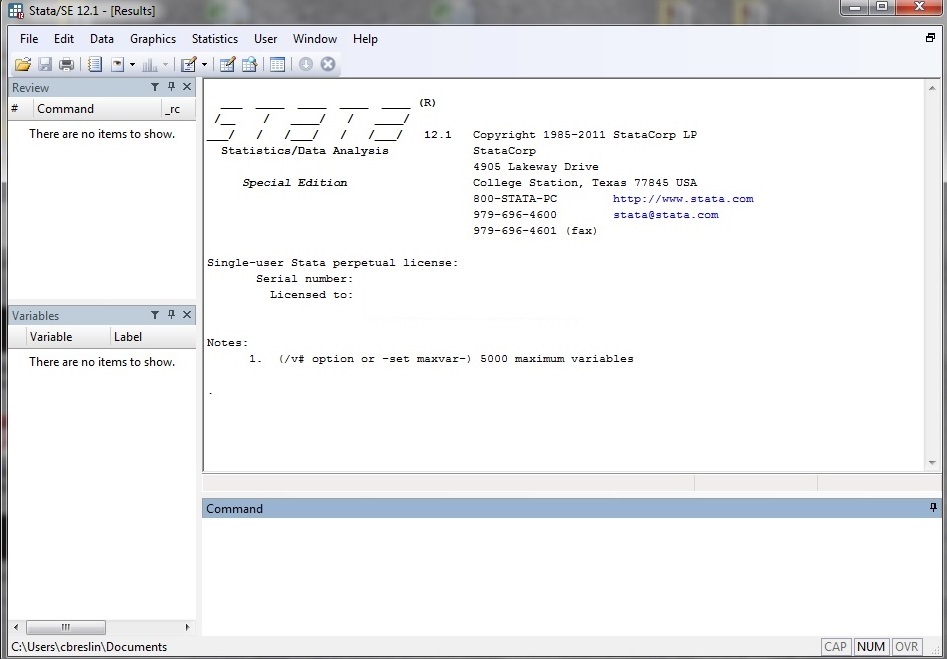
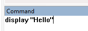
COMMAND: You can tell Stata what to do by typing in commands. Click inside the command window and type display “Hello”
RESULTS: Here Stata displays the commands followed by the output that Stata has produced. Note what appeared as the result of the command you just typed in.
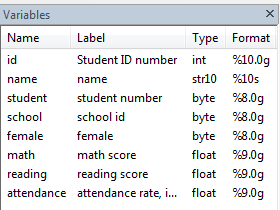
VARIABLES: lists all the variables in the dataset. The variable window can act as a shortcut for creating commands. Try clicking on one of the variables. It should appear in the command window, eliminating the need for you to write it out.
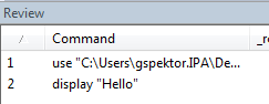
REVIEW: Lists all your prior commands. Notice that display “Hello!” now appears there. You can click on it and it will appear in your command window.
Useful tip: When you are in the command window, you can scroll through your previous commands using the Page Up and Page Down buttons on your keyboard.
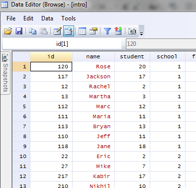
DATA EDITOR:Now let’s look at what a dataset stored in Stata actually looks like (the way Stata sees it and reads it). Type browse in the command window.
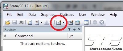
DO-FILE: Despite we can type codes directly in the Command window, it is a better idea to write all commands in the same file so be can save and reproduce them in the future. The set of commands we want Stata to execute can be saved in what Stata calls “do‐files”. Then, we will open the Do‐file editor by clicking the icon at the top of the screen.
We can start by typing clear all set more off so we clear our workspace and tell Stata to allow our screen to scroll (otherwise Stata will wait until we hit the button "more" to proceed with computations).
Some Basic Comments
1. Select directory
The first step will be to select the directory where we are going to work (i.e., the folder with the dataset and where Stata is going to save the files resulting from our work). Then, we are going to use the change directory command cd:
cd “c:/path” for Windows, or
cd “/Users/user_name/path” for Mac OS
Useful tip: When you are in the command window, you can type cd or pwd to know your current directory.
2. Importing Datasets into STATA
(i) To import datasets from STATA Example Datasets - use the command sysuse
E.g. sysuse auto.dta, clear -"auto" is one of the example datasets from STATA.
(ii) To import datasets from STATA Online Example Datasets - use the command webuse
E.g. webuse auto.dta, clear
(iii) To import datasets from local directory - use the command use
E.g. use "$dir/file.dta", clear
(iv) To import .csv file from local directory - use the command import delimited
E.g. import delimited "$dir/csv_file.csv", clear
(v) To import .xls or .xlsx file from local directory - use the command import excel
E.g. import excel "$dir/xlsx_file.xlsx", firstrow sheet(sheet_name) clear - "firstrow" is to use 1st row of the file as variables, "sheet()" is to import the particular sheet.
Useful tip: Use clear when you import the datasets to clear the previous memory.
3. Explore and summarize data
Please use the STATA example datasets for this exercise. The sysuse command loads a specified Stata-format dataset that was shipped with Stata. Here we will use the auto data file. E.g. sysuse auto.dta, clear
(i) describe
The describe command shows you basic information about a Stata data file. As you can see, it tells us the number of observations in the file, the number of variables, the names of the variables, and more.
describe
 Contains data from auto.dta
  obs:            74
 vars:            12                          17 Feb 1999 10:49
 size:         3,108 (99.6% of memory free)
-------------------------------------------------------------------------------
   1. make      str17  %17s
   2. price     int    %9.0g
   3. mpg       byte   %9.0g
   4. rep78     byte   %9.0g
   5. hdroom    float  %9.0g
   6. trunk     byte   %9.0g
   7. weight    int    %9.0g
   8. length    int    %9.0g
   9. turn      byte   %9.0g
  10. displ     int    %9.0g
  11. gratio    float  %9.0g
  12. foreign   byte   %9.0g
-------------------------------------------------------------------------------
Sorted by:
(ii) codebook
The codebook command is a great tool for getting a quick overview of the variables in the data file. It produces a kind of electronic codebook from the data file. Have a look at what it produces below.
codebook make price
 make -------------------------------------------------------------- (unlabeled)
                  type:  string (str17)

         unique values:  74                   coded missing:  0 / 74

              examples:  "Cad. Deville"
                         "Dodge Magnum"
                         "Merc. XR-7"
                         "Pont. Catalina"

               warning:  variable has embedded blanks

price ------------------------------------------------------------- (unlabeled)
                  type:  numeric (int)

                 range:  [3291,15906]                 units:  1
         unique values:  74                   coded missing:  0 / 74

                  mean:   6165.26
              std. dev:    2949.5

           percentiles:        10%       25%       50%       75%       90%
                              3895      4195    5006.5      6342     11385
(iii) inspect
Another useful command for getting a quick overview of a data file is the inspect command. Here is what the inspect command produces for the auto data file.
inspect mpg
mpg:                                           Number of Observations
------                                                             Non-
                                               Total   Integers    Integers
|      #                        Negative           -         -          -
|      #                        Zero               -         -          -
|      #                        Positive          74        74          -
|  #   #                                       -----     -----      -----
|  #   #   #                    Total             74        74          -
|  #   #   #   #   .            Missing            -
+----------------------                        -----
12                   41                           74
  (21 unique values)
(iv) list
The list command is useful for viewing all or a range of observations. Here we look at make, price, mpg, rep78 and foreign for the first 10 observations.
list make price mpg rep78 foreign in 1/10
                   make      price        mpg      rep78    foreign
  1.      Dodge Magnum       5886         16          2          0
  2.        Datsun 510       5079         24          4          1
  3.      Ford Mustang       4187         21          3          0
  4.  Linc. Versailles      13466         14          3          0
  5.     Plym. Sapporo       6486         26          .          0
  6.       Plym. Arrow       4647         28          3          0
  7.     Cad. Eldorado      14500         14          2          0
  8.        AMC Spirit       3799         22          .          0
  9.    Pont. Catalina       5798         18          4          0
 10.        Chev. Nova       3955         19          3          0
(v) tabulate
(a) The tabulate command is useful for obtaining frequency tables. Below, we make a table for rep78 and a table for foreign. The command can also be shortened to tab.
tabulate rep74
tab rep74
      rep78 |      Freq.     Percent        Cum.
------------+-----------------------------------
          1 |          2        2.90        2.90
          2 |          8       11.59       14.49
          3 |         30       43.48       57.97
          4 |         18       26.09       84.06
          5 |         11       15.94      100.00
------------+-----------------------------------
      Total |         69      100.00
tabulate foreign or tab foreign
     foreign |      Freq.     Percent        Cum.
------------+-----------------------------------
          0 |         52       70.27       70.27
          1 |         22       29.73      100.00
------------+-----------------------------------
      Total |         74      100.00
(b) The tab1 command can be used as a shortcut to request tables for a series of variables (instead of typing the tabulate command over and over again for each variable of interest).
tab1 rep74 foreign
 -> tabulation of rep78

      rep78 |      Freq.     Percent        Cum.
------------+-----------------------------------
          1 |          2        2.90        2.90
          2 |          8       11.59       14.49
          3 |         30       43.48       57.97
          4 |         18       26.09       84.06
          5 |         11       15.94      100.00
------------+-----------------------------------
      Total |         69      100.00

-> tabulation of foreign

    foreign |      Freq.     Percent        Cum.
------------+-----------------------------------
          0 |         52       70.27       70.27
          1 |         22       29.73      100.00
------------+-----------------------------------
      Total |         74      100.00
(c) We can use the plot option to make a plot to visually show the tabulated values.
tabulate rep78, plot
      rep78 |      Freq.
------------+------------+-----------------------------------------------------
          1 |          2 |**
          2 |          8 |********
          3 |         30 |******************************
          4 |         18 |******************
          5 |         11 |***********
------------+------------+-----------------------------------------------------
      Total |         69
(d) We can also make crosstabs using tabulate. Let’s look at the repair history broken down by foreign and domestic cars.
tabulate rep78 foreign
           |        foreign
     rep78 |         0          1 |     Total
-----------+----------------------+----------
         1 |         2          0 |         2
         2 |         8          0 |         8
         3 |        27          3 |        30
         4 |         9          9 |        18
         5 |         2          9 |        11
-----------+----------------------+----------
     Total |        48         21 |        69
(vi) summarize
(a) For summary statistics, we can use the summarize command. Let’s generate some summary statistics on mpg.
summarize mpg
Variable |     Obs        Mean   Std. Dev.       Min        Max
---------+-----------------------------------------------------
     mpg |      74     21.2973   5.785503         12         41
(b) We can use the detail option of the summarize command to get more detailed summary statistics.
summarize mpg, detail
                              mpg
-------------------------------------------------------------
      Percentiles      Smallest
 1%           12             12
 5%           14             12
10%           14             14       Obs                  74
25%           18             14       Sum of Wgt.          74

50%           20                      Mean            21.2973
                        Largest       Std. Dev.      5.785503
75%           25             34
90%           29             35       Variance       33.47205
95%           34             35       Skewness       .9487176
99%           41             41       Kurtosis       3.975005
(vii) mean
Let's generate the Mean, Std.Err, Conf.Interval (95%) for price and mpg
mean price mpg
Mean estimation                   Number of obs   =         74

--------------------------------------------------------------
             |       Mean   Std. Err.     [95% Conf. Interval]
-------------+------------------------------------------------
       price |   6165.257   342.8719      5481.914      6848.6
         mpg |    21.2973   .6725511       19.9569    22.63769
--------------------------------------------------------------
(viii) sort
The sort arranges the observations of the current data into ascending order based on the values of the variables in varlist.
sort price
     +-------+        +-------+
     | price |        | price |
     |-------|        |-------|
  1. | 4,099 |     1. | 3,291 |
  2. | 4,749 |     2. | 3,299 |
  3. | 3,799 | --> 3. | 3,667 |
  4. | 4,816 |     4. | 3,748 |
  5. | 7,827 |     5. | 3,798 |
     +-------+        +-------+
  Shown top 5 observations
(ix) gsort
The gsort arranges observations to be in ascending or descending order of the specified variables and so differs from sort in that sort produces ascending-order arrangements only.
gsort -price
     +-------+        +--------+
     | price |        | price  |
     |-------|        |--------|
  1. | 4,099 |     1. | 15,906 |
  2. | 4,749 |     2. | 14,500 |
  3. | 3,799 | --> 3. | 13,594 |
  4. | 4,816 |     4. | 13,466 |
  5. | 7,827 |     5. | 12,990 |
     +-------+        +--------+
  Shown top 5 observations
(x) order
The order command is used to reorder variables in dataset. Here we specify variable to be a first variable
order foreign
     +---------------------------------+          +---------------------------------------+
     | make                price   mpg |          | foreign     make                price |
     |---------------------------------|          |---------------------------------------|
  1. | Cad. Seville       15,906    21 |       1. | Domestic    Cad. Seville       15,906 |
  2. | Cad. Eldorado      14,500    14 |       2. | Domestic    Cad. Eldorado      14,500 |
  3. | Linc. Mark V       13,594    12 |  -->  3. | Domestic    Linc. Mark V       13,594 |
  4. | Linc. Versailles   13,466    14 |       4. | Domestic    Linc. Versailles   13,466 |
  5. | Peugeot 604        12,990    14 |       5. | Foreign     Peugeot 604        12,990 |
     +---------------------------------+          +---------------------------------------+
(xi) browse
Browse using Data Editor. The browse is a convenient alternative to list.
browse or br
(xii) generate
(a) The command generate creates a new variable. The values of the variable are specified by =exp.
generate or gen or g
E.g. generate new_var = 1
Operators is very important when we use if condition.
Operator
&       and;
|       or;
!=      not equal to // use "~="
==      equal when using 'if'
>       more than // >= more than or equal to
<       less than // <= less than or equal to
_n      row number
_N      total observations
  E.g. gen new_var1 = 1 if foreign == 1
       gen new_var2 = 1 if foreign == 1 & rep78 == 3
       gen new_var3 = 1 if foreign == 1 & rep78 != 3
(b) The command egen - Extensions to generate where depending on the function (fcn), arguments refers to an expression.
egen new_mean_var = mean(price)
(xiii) drop
Drop variables or observations. The command drop eliminates variables or observations from the data in memory.
drop price - to eliminate price variable from the dataset
drop price if price < 5000 - to eliminate price observations that are less than 5000 from the dataset
(xiv) keep
keep works the same way as drop, except that you specify the variables or observations to be kept rather than the variables or observations to be deleted.
keep price - to keep price variable only and drop all other variables from the dataset
keep price if price < 5000 - to keep price observations that are less than 5000