STATA 103
Alosias A, Behavioral Development Lab
STATA 103 introduces essential Stata concepts and shows how to practically apply them to a variety of data tasks. Let’s illustrate use of the process using example STATA auto dataset. sysuse auto, clear
1. locals and macros
Macros allow the user to store string information in temporary variables separate from the dataset. Macros are cleared from memory once the Stata session ends. Stata provides 2 types of macros, local and global, which differ in their scope (where they are available, see below).
To use macros, we assign a string to the macro name. Then, wherever the macro name is used elsewhere (in the do-file or program) with special substitution operators, Stata will directly substitute the string stored assigned to the macro.
See help macro for extensive documentation on macros.
(i) Global macros
Like their name suggests, global macros can be used anywhere. To substitute the contents of the global macro, precede the macro name with $. Here we store the string Hello world! in the global macro greeting. We then use display to print the string to screen. In place of $greeting below, Stata substitutes Hello world! (without quotes) — resulting in display "Hello world!".
Omitting the quotes in the display statement results in the substituted expression display Hello world!. Stata then interprets Hello as a variable name, which does not exist and causes an error.
global greeting Hello world!
global "$greeting"
Hello world!
One common usage of macros is to group variables together that are alike in some way. Here we group together a set of demographic variables whose names we store in a global macro. We then access the contents of the macro for the summary command.
global demographics price mpg rep78
summ $demographics
    Variable |        Obs        Mean    Std. Dev.       Min        Max
-------------+---------------------------------------------------------
       price |         74    6165.257    2949.496       3291      15906
         mpg |         74     21.2973    5.785503         12         41
       rep78 |         69    3.405797    .9899323          1          5
(ii) Local macros
Local macros have much more limited scope than globals. If declared inside a do-file or macro, the local macro is deleted after the do-file code has finished executed. For example, if declared in a do-file, the contents of the local macro cannot be accessed through typing commands in the Command window after the code has been executed.
The contents of local macros are accessed with the two single quotes ` and '. Here we group together a set of outcome variables and store them in a local macro, which we then use for summarize again.
local demographics price mpg rep78
summ `demographics'
    Variable |        Obs        Mean    Std. Dev.       Min        Max
-------------+---------------------------------------------------------
       price |         74    6165.257    2949.496       3291      15906
         mpg |         74     21.2973    5.785503         12         41
       rep78 |         69    3.405797    .9899323          1          5
(iii) tempfile
The tempfile assigns names to the specified local macro names that may be used as names for temporary files. When the program or do-file concludes, any datasets created with these assigned names are erased.
tempfile new_file
save `new_file', replace
This dataset has been saved temporarily within the do-file and that may be used anywhere in the same do-file. For e.g. use `new_file', clear
2. Looping
Loops are a programmer’s tool to perform some task repeatedly over a set of items.
The “for” loop is found in most programming languages, and is distinguished from other types of loops in that the programmer explicitly defines the items over which the for loop iterates (other types of loops run until some condition is met).
For loops come in 2 flavors in Stata: the forvalues loop, which iterates over set of numbers, and the foreach loop, which iterates over a general set of items (e.g. variable names).
(i) forvalues
The general syntax of a forvalues loop is this:
forvalues loop_name = range {
commands
}
- loop_name: the name of the loop control variable, a local macro, that takes on the values in range
- range: the range of values to loop over (e.g. 1/5 for 1 through 5, 2(2)10 for 2 through 10 in increments of 2
- commands: Stata commands to be run each time the loop iterates
- the opening { must be on the first line
- the closing } must be by itself on the last line
As we mentioned in the syntax description above, the loop control variable is a local macro, so its contents can be accessed with the usual local substitution operators ` and '. Here we display the contents of the loop control variable i for each iteration.
forvalues i = 1/5 {
display " i = `i' "
}
i = 1
i = 2
i = 3
i = 4
i = 5
(ii) foreach
The foreach loop expands on the types of lists over which the loop can iterate, including lists of strings, variable names, items in a global macro, etc. The syntax is similar, but slightly different from forvalues:
  foreach loop_name (in|of listtype) list  {
      commands
  }
- loop_name: tthe name of the loop control variable, a local macro, that takes on the values in list
- in: the keyword in is used if a generic list of items is specified
- of listtype: if using one of Stata’s specific types of lists, use the keyword of and one of the following listtypes (more are available):
- varlist: a list of variable names
- local: the contents of a local macro
- global: the contents of a globalmacro
- list: the list of values to loop over (e.g. 1/5 for 1 through 5, 2(2)10 for 2 through 10 in increments of 2
- commands: Stata commands to be run each time the loop iterates
- the opening { must be on the first line
- the closing } must be by itself on the last line
  foreach var of varlist price mpg rep78 {
      egen std_`var' = std(`var')
  }
    Variable |        Obs        Mean    Std. Dev.       Min        Max
-------------+---------------------------------------------------------
   std_price |         74   -4.83e-10           1  -.9744909   3.302511
     std_mpg |         74   -7.00e-09           1  -1.606999    3.40553
   std_rep78 |         69    8.64e-10           1  -2.430264   1.610416
3. Collapse
Sometimes you have data files that need to be collapsed to be useful to you. For example, you might have student data but you really want classroom data, or you might have weekly data but you want monthly data, etc.
Consider the collapse command below.
collapse price
     +---------+
     |   price |
     |---------|
  1. | 6,165.3 |
     +---------+
Useful tip: Once collapsed the dataset, you will not have same dataset structure. In this case, you might need to import the dataset again.
collapse price, by(foreign)
      +--------------------+
     |  foreign     price |
     |--------------------|
  1. | Domestic   6,072.4 |
  2. |  Foreign   6,384.7 |
     +--------------------+
collapse (mean)price (max)mpg (min)rep78, by(foreign)
      +----------------------------------+
     |  foreign     price   mpg   rep78 |
     |----------------------------------|
  1. | Domestic   6,072.4    34       1 |
  2. |  Foreign   6,384.7    41       3 |
     +----------------------------------+
4. preserve & restore
The command preserve preserves the data, guaranteeing that data will be restored after program termination.
The command restore forces a restore of the data now.
This will be useful to seperate a single dataset into multiple data files for analysis.
    sysuse auto, clear

    preserve

      drop make price mpg rep78
      save part1_dataset.dta, replace

    restore

    preserve

      collapse (mean)price (mean)mpg, by(foreign)
      save part2_dataset.dta, replace

    restore
sysuse auto, clear preserve drop make price mpg rep78 save part1_dataset.dta, replace restore preserve collapse (mean)price (mean)mpg, by(foreign) save part2_dataset.dta, replace restore
5. append & merge
(i) append
Append is used when you want to combine datasets that contain the same variables, but have different cases, thus, you are adding new rows to the dataset, but the number of columns should remain the same.
When you have two data files, you may want to combine them by stacking them one on top of the other. For example, we have a file containing dataset1 and a file containing dataset2 as shown below.
a) Data 1
input id x y
1 1 2
2 1 2
3 1 2
end
save dataset1, replace
list
     +------------+
     | id   x   y |
     |------------|
  1. |  1   1   2 |
  2. |  2   1   2 |
  3. |  3   1   2 |
     +------------+
b) Data 2
clear
input id y z
1 2 3
2 2 3
3 2 3
end
save dataset2, replace
list
     +------------+
     | id   y   z |
     |------------|
  1. |  1   2   3 |
  2. |  2   2   3 |
  3. |  3   2   3 |
     +------------+
If we wanted to combine these files by stacking them one atop the other, we can use the append command as shown below. While appending datasets, it appends with the same or matched varaibles and others will be shown as missing values.
input id x y 1 1 2 2 1 2 3 1 2 end save dataset1, replace list
clear input id y z 1 2 3 2 2 3 3 2 3 end save dataset2, replace list
use dataset1, clear
append using dataset2
We can use the list command to see if this worked correctly.
list
     +----------------+
     | id   x   y   z |
     |----------------|
  1. |  1   1   2   . |
  2. |  2   1   2   . |
  3. |  3   1   2   . |
  4. |  1   .   2   3 |
  5. |  2   .   2   3 |
  6. |  3   .   2   3 |
     +----------------+
(ii) merge
Merging is another way of combining datasets. Where the append command adds rows, or observations, merge adds columns, or variables. Thus, you would use merge when there are the same observations across datasets, with different variables, and you want to combine those datasets into one larger dataset.
Syntax
    One-to-one merge on specified key variables

        merge 1:1 varlist using filename [, options]


    Many-to-one merge on specified key variables

        merge m:1 varlist using filename [, options]


    One-to-many merge on specified key variables

        merge 1:m varlist using filename [, options]
(a) ONE-TO-ONE MERGE (1:1):
A 1-to-1 merge combines datasets that have identifiers for single observations in each dataset. In this type of merge, Stata combines the data based on those identifiers. In the example, we will be using dataset1 and dataset2, the variable “id” is unique to each observation, and present in each dataset.
Here is an example of a 1-to-1 merge:
clear
use dataset1, replace
merge 1:1 id using dataset2

list
      dataset1                   dataset2                                  merged dataset
   +------------+             +------------+                     +------------------------------+
   | id   x   y |             | id   y   z |                     | id   x   y   z        _merge |
   |------------|      +      |------------|       =             |------------------------------|
1. |  1   1   2 |          1. |  1   2   3 |                  1. |  1   1   2   3   matched (3) |
2. |  2   1   2 |          2. |  2   2   3 |                  2. |  2   1   2   3   matched (3) |
3. |  3   1   2 |          3. |  3   2   3 |                  3. |  3   1   2   3   matched (3) |
   +------------+             +------------+                     +------------------------------+
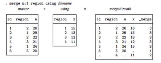
(b) MANY-TO-ONE (m:1) You would use a many-to-1 merge when you have a master dataset that has individual level data and using dataset that contains within-individual level data as well as a unique individual level identifier from the master data. The Stata merge gives this example of adding regional level data to person-level data:
(c) ONE-TO-MANY (1:m)
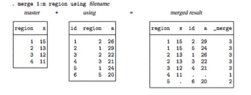
The one-to-many merge is simply the reverse of a many-to-one merge. In this case the master dataset would have within-individual level data and the using data would contain individual level data that you want to add to the master dataset. The Stata merge gives another example of adding person-level data, to regional level data:
6. reshape
The reshape command converts the data from wide to long form and vice versa. Before using reshape, you need to determine whether the data are in long or wide form. You also must determine the logical observation (i) and the subobservation (j) by which to organize the data.
 Syntax:
         long                                wide
        +---------------+                   +------------------+
        | i   j   a   b |                   | i   a1 a2  b1 b2 |
        |---------------| <--- reshape ---> |------------------|
        | 1   1   1   2 |                   | 1   1   3   2  4 |
        | 1   2   3   4 |                   | 2   5   7   6  8 |
        | 2   1   5   6 |                   +------------------+
        | 2   2   7   8 |
        +---------------+

        long to wide: reshape wide a b, i(i) j(j)    (j existing variable)
        wide to long: reshape long a b, i(i) j(j)    (j    new   variable)
Source:
(1) UCLA: https://stats.idre.ucla.edu/stata/
(1) UCLA: https://stats.idre.ucla.edu/stata/