STATA - Working with Map and Geo-Distance
A. Working with spmap and maps
How do I graph data onto a map with Stata?
With spmap, you can graph data onto maps and produce results. Obtain and install the spmap, shp2dta, and mif2dta commands and search the web for the files that describe the map onto which you want to graph your data. You can use ESRI shapefiles or MapInfo Interchange Format.
1. Install the spmap, shp2dta, and mif2dta commands
ssc install spmap
ssc install shp2dta
ssc install mif2dta
Syntax:
spmap [attribute] [if] [in] using basemap [, id(idvar) basemap_options]
shp2dta using shpfilename, database(filename) coordinates(filename) [options]
mif2dta using miffile [, type(spobj) genid(idvar) options]
Important Note: This works only on STATA version 15.1 and above versions.
2. Find a map (as ESRI shapefile or a Mapinfo format file).
A map recordes the geometry and attribute information of spatial features. Those maps are available from public or provate sources. You will want a "polygon shapefile". The map is stored in these files:
.shp
.shx
.dbf
.mif
We are going to use Nepal Country Map shapefile to find poverty level in each state by merging Poverty dataset. Please download the example dataset here: a) Nepal Shapefiles (shape_files_of_districts_in_nepal.rar) - Please unzip it - we need only .shp and .dbf files b) Poverty Dataset (poverty.dta)
Useful tip: Free Downloadable GIS Shapfiles Avabilable from these (private) Website:
1. DIVA-GIS free, simple & effective - http://www.diva-gis.org/gdata
2. STAT Silk - https://www.statsilk.com/maps/download-free-shapefile-maps
3. Free GIS Data - https://freegisdata.rtwilson.com/
3. Converting Shapefile into Stata file.
We use shp2dta command to extract data from shapefile in the curernt directory.
shp2dta using shape_files_of_districts_in_nepal, database(nepaldb) coordinates(nepalcoord) genid(id)
Pay attention to the three options we specified:
- database(nepaldb) specified that we wanted the database file to be named nepaldb.dta.
- coordinates(nepalcoord) specified that we wanted the coordinate file to be named nepalcoord.dta.
- genid(id) specified that we wanted the ID variable created in nepaldb.dta to be named id.
4. Let's look at the data structure.
a) Nepal Dataset (extracted from the map)
use nepaldb, clear

describe

Contains data from nepaldb.dta
  obs:            75
 vars:            11                          18 Jan 2022 14:17
 size:         3,300
------------------------------------------------------------------------------------------------------------
              storage   display    value
variable name   type    format     label      variable label
------------------------------------------------------------------------------------------------------------
descriptio      str1    %9s                   descriptio
name            str1    %9s                   name
objectid        byte    %10.0g                objectid
dist_code       byte    %10.0g                dist_code
dist_name       str14   %14s                  dist_name
shape_area      double  %10.0g                shape_area
shape_len       double  %10.0g                shape_len
cartodb_id      byte    %10.0g                cartodb_id
created_at      long    %12.0g                created_at
updated_at      long    %12.0g                updated_at
id              byte    %12.0g
------------------------------------------------------------------------------------------------------------
Sorted by: id
b) Napel Coordinate data (extracted from the map)
use nepalcoord, clear

describe

Contains data from nepalcoord.dta
  obs:        55,251
 vars:             3                          18 Jan 2022 14:17
 size:       939,267
-------------------------------------------------------------------------------------------------------------
              storage   display    value
variable name   type    format     label      variable label
-------------------------------------------------------------------------------------------------------------
_ID             byte    %12.0g
_X              double  %10.0g
_Y              double  %10.0g
-------------------------------------------------------------------------------------------------------------
Sorted by: _ID
c) Poverty dataset
use poverty, clear

describe

Contains data from poverty.dta
  obs:            75
 vars:             3                          18 Nov 2020 12:55
 size:         1,725
---------------------------------------------------------------------------------------------------------------
              storage   display    value
variable name   type    format     label      variable label
---------------------------------------------------------------------------------------------------------------
ID              byte    %10.0g                ID
dist_name       str14   %14s                  District
poverty         double  %10.0g                poverty
---------------------------------------------------------------------------------------------------------------
Sorted by:
use nepaldb, clear
describe
use nepalcoord, clear
describe
use poverty, clear
describe
5. Merge Datasets
use nepaldb, clear

merge 1:1 dist_name using poverty

    Result                           # of obs.
    -----------------------------------------
    not matched                             0
    matched                                75  (_merge==3)
    -----------------------------------------
use nepaldb, clear
merge 1:1 dist_name using poverty
6. Draw the graph
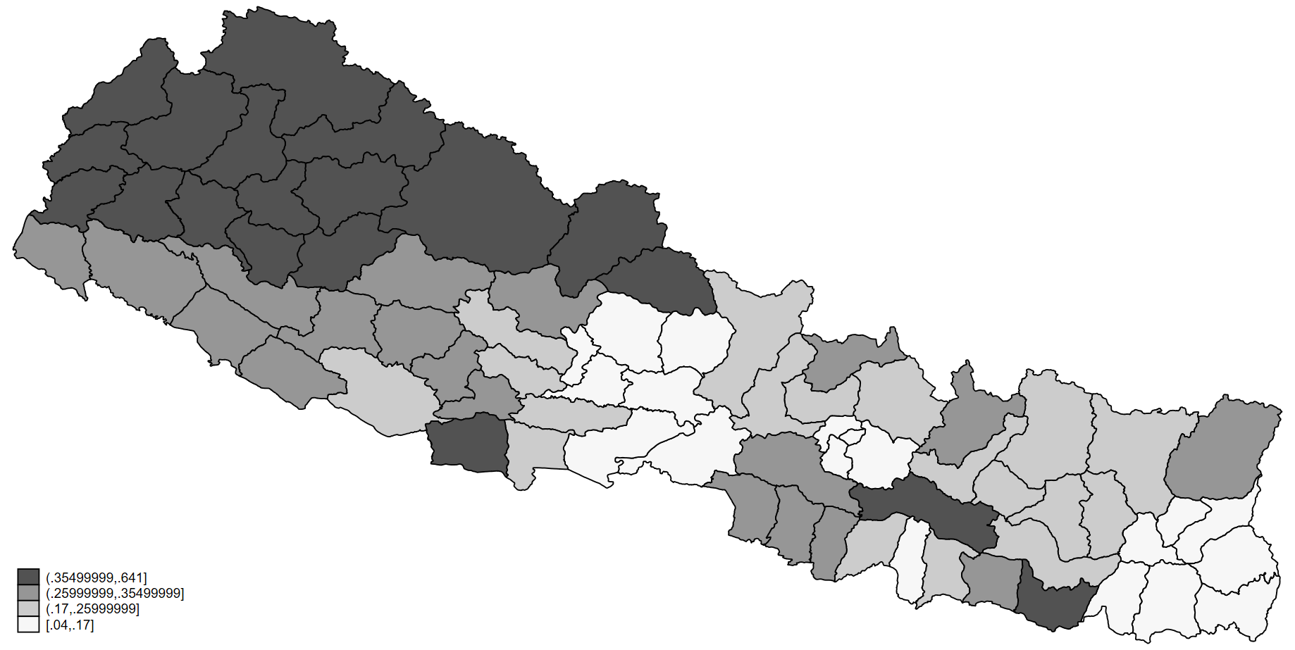
spmap poverty using nepalcoord, id(id)
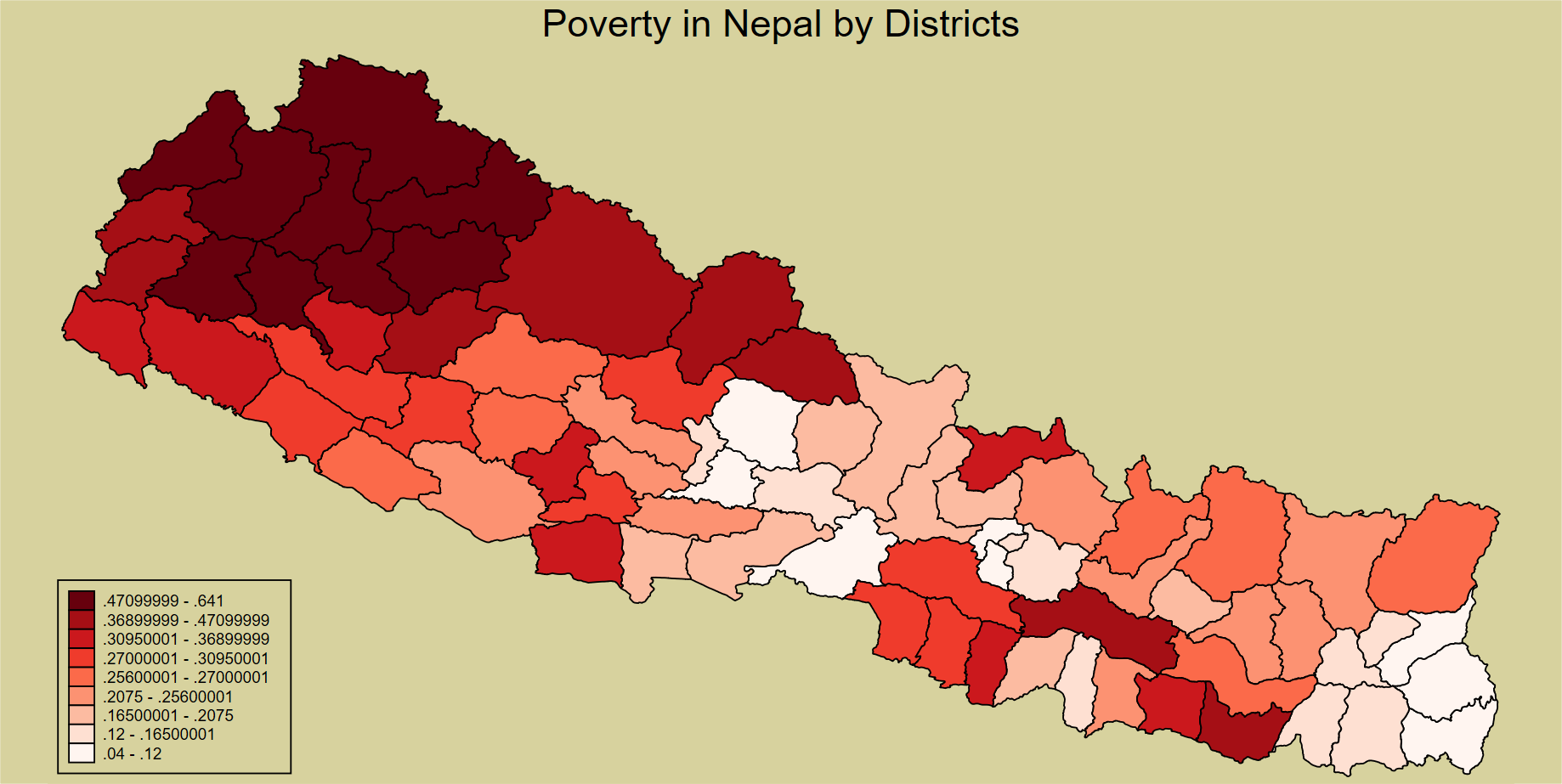
Adding Title, Legends and Colors to the base map based on the povery level
spmap poverty using nepalcoord, id(id) ///
title ("Poverty in Nepal by Districts") ///
fcolor(Reds) ///
clnumber(9) ///
legstyle(2) ///
legend(region(lcolor(black))) ///
plotregion(icolor(stone)) ///
graphregion(icolor(stone))
    Notes:

    title ("Title")               - graph title
    fcolor(Reds)                  - fill color of base map polygons (using Reds pallets here)
                                    We can use Blues, Greens or others.
    clnumber(9)                   - number of classes or number of color legends
    legstyle(2)                   - base map legend style
    legend(region(lcolor(black))) - legend region line color
    plotregion(icolor(stone))     - plot region color
    graphregion(icolor(stone))    - graph region color
spmap has many options that control the color, legend, etc. Read about them in the online help file (type help spmap).
B. Working with Geo-Distance
Part 1: How do I calculate the distance between two locations with Stata?
The geodist command is used to calculate the distance between two locations, cities or latitude and longitude.
1. Please install geodist if you haven't installed this command.
ssc install geodist
Syntax: geodist lat1 lon1 lat2 lon2 [if] [in] , generate(new_dist_var) [options]2. Import latitude and longitude data
The data that we are going to use, is us_cities.dta that contains latitude and longitude of US cities.
use "us_cities.dta", clear
describe
Contains data from distance.dta
  obs:           726
 vars:             3                          1 Jun 2020 11:17
 size:        58,806
---------------------------------------------------------------------------------------------------------------
              storage   display    value
variable name   type    format     label      variable label
---------------------------------------------------------------------------------------------------------------
city            str65   %65s
latitude        double  %10.0g
longitude       double  %10.0g
---------------------------------------------------------------------------------------------------------------
Sorted by:
list in 1/5
     +----------------------------------------+
     |          city    latitude    longitude |
     |----------------------------------------|
  1. |        Dallas   32.778155   -96.795404 |
  2. | New York City   40.697132   -73.931351 |
  3. |      Triangle   38.544054   -77.343246 |
  4. |    Long Beach   33.766725    -118.1924 |
  5. | San Francisco   37.755363   -122.44335 |
     +----------------------------------------+
3. Find Distance between Cities We are going to generate the distance between New York and other cities in KM. New York's Lat = 40.697132 and Log = -73.931351 which can be found in row 2 (highlighted below) and calculating distance with other cities from New York city using variables latitude and longitude.
       +----------------------------------------+
       |          city    latitude    longitude |
       |----------------------------------------|
    1. |        Dallas   32.778155   -96.795404 |
  +-------------------------------------------------+
  | 2. | New York City   40.697132   -73.931351 |   |
  +-------------------------------------------------+
    3. |      Triangle   38.544054   -77.343246 |
    4. |    Long Beach   33.766725    -118.1924 |
    5. | San Francisco   37.755363   -122.44335 |
       +----------------------------------------+
Syntax: geodist lat1 lon1 lat2 lon2 [if] [in] , generate(new_dist_var) [options]
geodist 40.697132 -73.931351 latitude longitude, generate(km)
list in 1/5
     +----------------------------------------------------+
     |          city    latitude    longitude          km |
     |----------------------------------------------------|
  1. |        Dallas   32.778155   -96.795404   2214.6893 |
  2. | New York City   40.697132   -73.931351           0 |
  3. |      Triangle   38.544054   -77.343246   378.06096 |
  4. |    Long Beach   33.766725    -118.1924   3959.4835 |
  5. | San Francisco   37.755363   -122.44335   4148.4027 |
     +----------------------------------------------------+
This calculates the distance in Kilo Meter (KM) by default. If you would like to calcualte the distance in Miles, simply add mile as option. geodist 40.697132 -73.931351 latitude longitude, gen(mile) mile
list in 1/5
     +----------------------------------------------------------------+
     |          city    latitude    longitude          km        mile |
     |----------------------------------------------------------------|
  1. |        Dallas   32.778155   -96.795404   2214.6893   1376.1441 |
  2. | New York City   40.697132   -73.931351           0           0 |
  3. |      Triangle   38.544054   -77.343246   378.06096   234.91619 |
  4. |    Long Beach   33.766725    -118.1924   3959.4835    2460.309 |
  5. | San Francisco   37.755363   -122.44335   4148.4027   2577.6979 |
     +----------------------------------------------------------------+
Use sphere option for Haversine formula (Default is Vincenty's (1975) formula) to calculate the distance in km/miles. geodist 40.697132 -73.931351 latitude longitude,gen(km2) sphere
list in 1/5
     +----------------------------------------------------------------------------+
     |          city    latitude    longitude          km        mile         km2 |
     |----------------------------------------------------------------------------|
  1. |        Dallas   32.778155   -96.795404   2214.6893   1376.1441   2211.0716 |
  2. | New York City   40.697132   -73.931351           0           0           0 |
  3. |      Triangle   38.544054   -77.343246   378.06096   234.91619   377.72721 |
  4. |    Long Beach   33.766725    -118.1924   3959.4835    2460.309   3950.8549 |
  5. | San Francisco   37.755363   -122.44335   4148.4027   2577.6979    4138.325 |
     +----------------------------------------------------------------------------+
We can sort km/mile/km2 variable to find the nearest city to New York City. sort km
list in 1/5
     +----------------------------------------------------------------------------+
     |          city    latitude    longitude          km        mile         km2 |
     |----------------------------------------------------------------------------|
  1. | New York City   40.697132   -73.931351           0           0           0 |
  2. |       Hoboken    40.74617   -74.032814   10.155831   6.3105406   10.141295 |
  3. |     Weehawken   40.766387   -74.025431    11.05931   6.8719369   11.051845 |
  4. |   Jersey City   40.717892   -74.067467   11.731366   7.2895326   11.703296 |
  5. |        Inwood      40.616   -73.746614   18.034896   11.206365   18.006539 |
     +----------------------------------------------------------------------------+
Part 2: How do I find the nearest city/location with Stata?
The geodist or geonear command is used to find the nearest city or area by calculating the distance.
1. Please install geodist and geonear if you haven't installed this command.
ssc install geodist
ssc install geonear
Syntax:
geodist lat1 lon1 lat2 lon2 [if] [in] , generate(new_dist_var) [options]
geonear baseid baselat baselon using nborfile , neighbors(nborid nborlat nborlon) [options]
geodist and geonear commands will help to find the nearest city or location. Now, let us see how to use both commands to find the nearest cities or locations. Let's use the US Industrial cities data, please download the us_industrial_cities.dta dataset that contains 4 US industrial cities locations.
2. Method 1: Using geodist
use "us_industrial_cities.dta", clear
describe
Contains data from industrialcities.dta
  obs:             4
 vars:             3                          1 Jun 2020 11:18
 size:           324
---------------------------------------------------------------------------------------------------------------
              storage   display    value
variable name   type    format     label      variable label
---------------------------------------------------------------------------------------------------------------
city1           str65   %65s
latitude1       double  %10.0g
longitude1      double  %10.0g
---------------------------------------------------------------------------------------------------------------
Sorted by:
Note: cross command is used for pairwise combination. Please make sure to have different variable names in the both files.
cross using "us_cities.dta"
Let's keep city distance that is less than 10 kms.Syntax: geodist lat1 lon1 lat2 lon2 [if] [in] , generate(new_dist_var) [options]
geodist latitude longitude latitude1 longitude1, gen(distance)
bysort city1 (distance): keep if distance<10
     +------------------------------------------------------------------------------------+
     |   city1   latitude1   longitude1         city    latitude    longitude    distance |
     |------------------------------------------------------------------------------------|
  1. |  Boston     42.3505   -71.105399       Boston     42.3505   -71.105399           0 |
  2. |  Boston     42.3505   -71.105399    Brookline   42.331779   -71.121182   2.4527659 |
  3. |  Boston     42.3505   -71.105399   Somerville   42.386675   -71.098264    4.061087 |
  4. |  Boston     42.3505   -71.105399     Brighton   42.350097   -71.156442   4.2059165 |
  5. |  Boston     42.3505   -71.105399      Medford   42.407484   -71.119023   6.4284976 |
     |------------------------------------------------------------------------------------|
  6. |  Boston     42.3505   -71.105399    Watertown   42.370888   -71.182911   6.7752439 |
  7. |  Boston     42.3505   -71.105399       Revere    42.40807   -71.013589   9.9028531 |
  8. | Chicago   41.842602   -87.681229      Chicago   41.842602   -87.681229           0 |
  9. | Chicago   41.842602   -87.681229       Cicero    41.84484   -87.746834   5.4543704 |
 10. | Houston   29.813822   -95.365295      Houston   29.813822   -95.365295           0 |
     +------------------------------------------------------------------------------------+
3. Method 2: Using geodnearSyntax: geonear baseid baselat baselon using nborfile , neighbors(nborid nborlat nborlon) [options]
use "us_cities.dta", clear
geonear city latitude longitude using "us_industrial_cities.dta", n(city1 latitude1 longitude1) ignoreself
list in 1/5
     +------------------------------------------------------------+
     |      city    latitude    longitude         nid   km_to_nid |
     |------------------------------------------------------------|
  1. |     Afton   38.550245   -90.332723   Iowa City    360.1443 |
  2. |    Aguada   18.379626   -67.188421      Boston   2691.0149 |
  3. | Aguadilla   18.429675   -67.155179      Boston   2685.9266 |
  4. |  Aibonito    18.13996      -66.266      Boston   2730.7248 |
  5. |     Akron   41.084195   -81.514059     Chicago   520.64629 |
     +------------------------------------------------------------+
Note: 1. nid is nearest city for variable city in this output - Eg. The nearest city of 'Afton' is 'Iowa City'.
2. ignoreself is to ignore the self option - Eg. If city == "Boston" and nearest city (nid) == "Boston" which is km_to_nid = 0, this ignoreself option will drop the observation automaticaly from the output data.
Using us_industrial_cities.dta as our base cities to find nearest cities to the industrial cities.
use "us_industrial_cities.dta", clear
geonear city1 latitude1 longitude1 using "us_cities.dta", n(city latitude longitude) ignoreself
list in 1/4
     +------------------------------------------------------------+
     |     city1   latitude1   longitude1         nid   km_to_nid |
     |------------------------------------------------------------|
  1. |    Boston     42.3505   -71.105399   Brookline   2.4527762 |
  2. |   Chicago   41.842602   -87.681229      Cicero   5.4401878 |
  3. |   Houston   29.813822   -95.365295     Webster   39.218636 |
  4. | Iowa City   41.657825   -91.526534     Anamosa   53.932938 |
     +------------------------------------------------------------+
Use nearcount() to get the number of nearest cities. Let's get the first and second nearest cities.
use "us_industrial_cities.dta", clear
geonear city1 latitude1 longitude1 using "us_cities.dta", n(city latitude longitude) ignoreself nearcount(2)
list in 1/4
     +---------------------------------------------------------------------------------------+
     |     city1   latitude1   longitude1        nid1   km_to_n~1           nid2   km_to_n~2 |
     |---------------------------------------------------------------------------------------|
  1. |    Boston     42.3505   -71.105399   Brookline   2.4527762     Somerville   4.0649609 |
  2. |   Chicago   41.842602   -87.681229      Cicero   5.4401878   Bedford Park   13.930936 |
  3. |   Houston   29.813822   -95.365295     Webster   39.218636       Freeport   96.122487 |
  4. | Iowa City   41.657825   -91.526534     Anamosa   53.932938       Eldridge   78.253819 |
     +---------------------------------------------------------------------------------------+
The output data will show in wide format by default. To convert or show the output data in long format, use the option long.use "us_industrial_cities.dta", clear
geonear city1 latitude1 longitude1 using "us_cities.dta", n(city latitude longitude) ignoreself nearcount(2) long
list in 1/8
     +--------------------------------------+
     |     city1           city   km_to_c~y |
     |--------------------------------------|
  1. |    Boston      Brookline   2.4527762 |
  2. |    Boston     Somerville   4.0649609 |
  3. |   Chicago         Cicero   5.4401878 |
  4. |   Chicago   Bedford Park   13.930936 |
  5. |   Houston        Webster   39.218636 |
  6. |   Houston       Freeport   96.122487 |
  7. | Iowa City        Anamosa   53.932938 |
  8. | Iowa City       Eldridge   78.253819 |
     +--------------------------------------+
Use within(10) to get the cities within 10km of the base city. Within can only be used with long option.
use "us_industrial_cities.dta", clear
geonear city1 latitude1 longitude1 using "us_cities.dta", n(city latitude longitude) ignoreself long within(10)
list in 1/9
     +------------------------------------+
     |     city1         city   km_to_c~y |
     |------------------------------------|
  1. |    Boston    Brookline   2.4527762 |
  2. |    Boston   Somerville   4.0649609 |
  3. |    Boston     Brighton   4.1948253 |
  4. |    Boston      Medford   6.4343941 |
  5. |    Boston    Watertown   6.7601531 |
     |------------------------------------|
  6. |    Boston       Revere   9.8918812 |
  7. |   Chicago       Cicero   5.4401878 |
  8. |   Houston      Webster   39.218636 |
  9. | Iowa City      Anamosa   53.932938 |
     +------------------------------------+
Note: 1. Use nearcount(0) will excluded the base cities that don't have neighbors within the specified distance. You can notice that 'Houston' and 'Iowa City' don't have neighbors within 10km. If you use nearcount(0), it will exclude them from the dataset.
2. By default, Stata will interpret within(10) as indicating cities within 10km. If we were to add a miles option, this would be interpreted as 10 miles.
Use limit() to limit the number of nearest cities to the base cities. Let's limit to 2 cities.
use "us_industrial_cities.dta", clear
geonear city1 latitude1 longitude1 using "us_cities.dta", n(city latitude longitude) ignoreself long nearcount(0) within(10) limit(2)
list in 1/4
     +------------------------------------+
     |   city1           city   km_to_c~y |
     |------------------------------------|
  1. |  Boston      Brookline   2.4527762 |
  2. |  Boston     Somerville   4.0649609 |
  3. | Chicago         Cicero   5.4401878 |
  4. | Chicago   Bedford Park   13.930936 |
     +------------------------------------+